2730
Deep learning Based Liver Segmentation from MR Images Using 3D Mutli-Resolution Convolutional Neural NetworksMootaz Eldib1 and Jonathan Riek1
1BioTelemetry Research, Rochester, NY, United States
Synopsis
A deep learning based image segmentation algorithm is presented for the liver in volumetric MRI data. The fully automated state-of-the-art algorithm was trained with a large dataset resulting in excellent segmentation accuracy as compared to the trained radiologist performance.
Introduction
MR imaging of the liver has several clinical applications that can provide quantitative biomarkers for disease including measurements of liver fat fraction, fibrosis, iron content, and liver volume [1][2]. To compute such biomarkers in the liver, a radiologist outlines the borders of the liver manually, which is laborious and introduces variability. To this end, several image-processing-based algorithms have been developed with varying degrees of accuracy to automate this task [3]. Due to recent advances in algorithms and hardware, deep learning approaches have been widely used for classification, including medical imaging segmentation problems [4]. In this abstract we exploit deep learning, specifically convolutional neural networks (CNN), for liver segmentation in MR images.Methods
A total of 220 scans were used for training, validation, and testing divided into 140, 30, and 50 scans for each part respectively. Data was collected on GE, Philips, and Siemens scanners using an axial T1-weighted spoiled gradient echo sequence with a TE of 1.15 and 2.3 ms for 3T scanners or 2.3 and 4.6 ms for 1.5 T scanners, TR = 150 ms, and flip angle of 9°. Complete coverage of the liver often required between one and four overlapping scans, which were stitched into a single three-dimensional dataset. Then, a radiologist identified the boundaries of the liver to generate labels for each voxel in the volume. The images and the labels were then resampled to a common spacing of 2x2x10 mm. Finally, the images were normalized to a mean of 0 and a variance of 1 before inserting them at the input layer of our network shown in Figure 1. For the network to learn the contextual information in the images, a multi-resolution approach was used at the input layer where the input segment was upsampled by a factor of 3 and 6 to generate two additional convolutional pathways [5]. The network consisted of 9 convolutional layers with feature maps of size [30, 30, 30, 40, 40, 40, 40, 50, and 50] per each pathway for feature extraction using 3x3x3 kernels. The Parametric Rectified Linear Unit was used as an activation function. At the last convolutional layer of the two sub-sampled pathways, the feature maps were resampled linearly before connecting into the fully connected layers. The fully connected hidden layers, which were used to compute the class score, had feature maps of size [150,150,and 150] convolved with kernels of size 1x1x1. The final classification layer computes the probability of each class (i.e. liver or not liver) using the Softmax classifier defined as $$$p_c (x)=exp(z_c (x) )/∑^c exp(z_c (x) ) $$$ where $$$c$$$ is the class of the voxel and $$$z_c (x)$$$ is the feature map activation at that voxel $$$x∈R^3$$$. Training was performed for 35 epochs using the Adam optimization and L1 and L2 regularization on GPU. Evaluation of the accuracy of the classification was compared to the ground truth radiologist segmentation using the Dice coefficient computed by $$$|Y_R ∩ Y_C |/(|Y_R |+|Y_C/Y_R |)$$$ where $$$Y_R$$$ is the radiologist’s segmentation and $$$Y_C$$$ is that generated from the proposed automated algorithm.Results
The convergence of the CNN is shown in Figure 2. The Dice coefficient of the validation data during training is plotted over the training epochs, which shows a rapid increase in the segmentation accuracy until approximately the 6th epoch followed by slower improvement thereafter. A Dice coefficient of 0.96 was obtained after 35 epochs of training. Similarly, for the testing data, the average Dice coefficient was 0.95±0.0081. The average volume of all the livers in the training set was 2387±594 ml and 2397±607 ml for the radiologist and CNN-based segmentations, respectively. The Dice coefficient for each liver is shown in Figure 3, demonstrating the high degree of accuracy achieved by the proposed method. A Bland-Altman plot comparing the automated segmentation to the manual segmentation is shown in Figure 4 indicating a small bias of 10.1 ml (0.4%) and only three livers outside of the 95% confidence limits. A Student’s T-test demonstrates no significant difference between the volumes derived from the two different segmentations (p=0.49). Finally, Figure 5 shows two examples of the resulting segmentation from the CNN segmentation as compared to the ground truth radiologist segmentation showing good visual agreement between the masks.Conclusions
In this study, we utilized a large dataset of manually segmented liver MR images to train a deep learning model to segment the liver automatically. Our initial findings indicate high agreement between that proposed method and the ground truth segmentation making it a viable method to automatically quantify MR-based liver biomarkers.Acknowledgements
No acknowledgement found.References
[1] B. Taouli,et al. American Journal of Roentgenology, vol. 193, no. 1. pp. 14–27, 2009.
[2] S. K. Venkatesh, et al. Magnetic Resonance Imaging Clinics of North America, vol. 22, no. 3. pp. 433–446, 2014.
[3] A. Gotra, et al. Insights Imaging, vol. 8, no. 4, pp. 377–392, 2017.
[4] M. Lai, arXiv cs.LG, vol. 5, p. 2000, 2015.
[5] K. Kamnitsas, et al. Med. Image Anal., vol. 36, pp. 61–78, 2017.
Figures
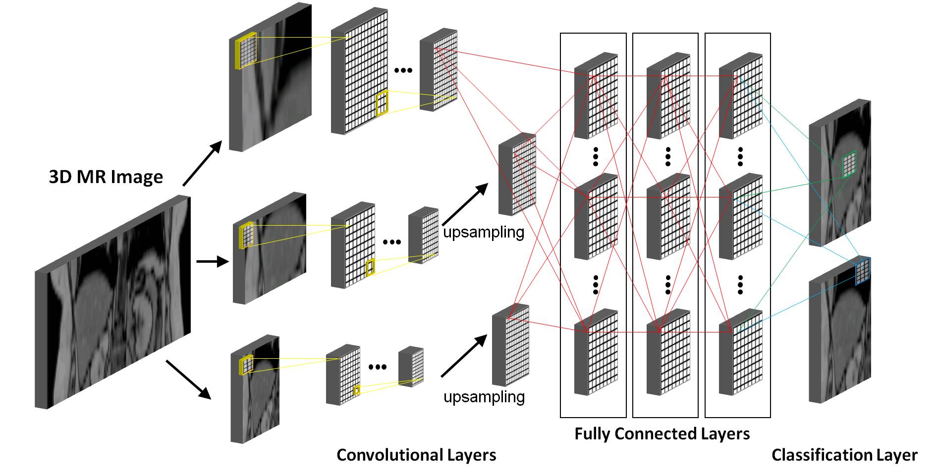
Graphical
representation of the convolutional neural network (CNN) used for the liver segmentation task. Our network
consisted of 9 convolutional layers for feature extraction followed by 3 fully
connected layers to compute the class scores. The final classification layer
outputs the final classification maps.
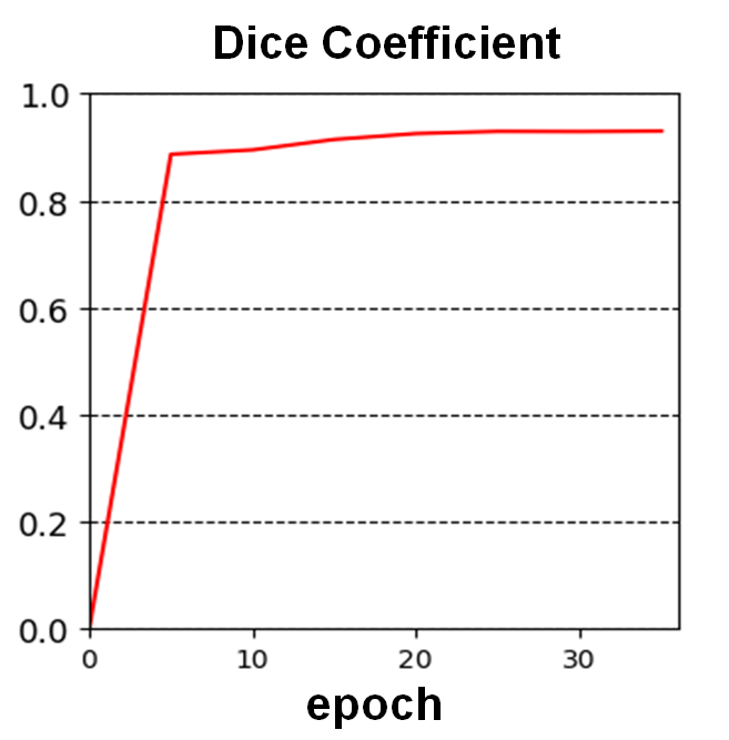
Plot of the Dice
coefficient over the training epochs.
The network parameters are plateaus after approximately 6 epochs but
continues to increase slowly after that.
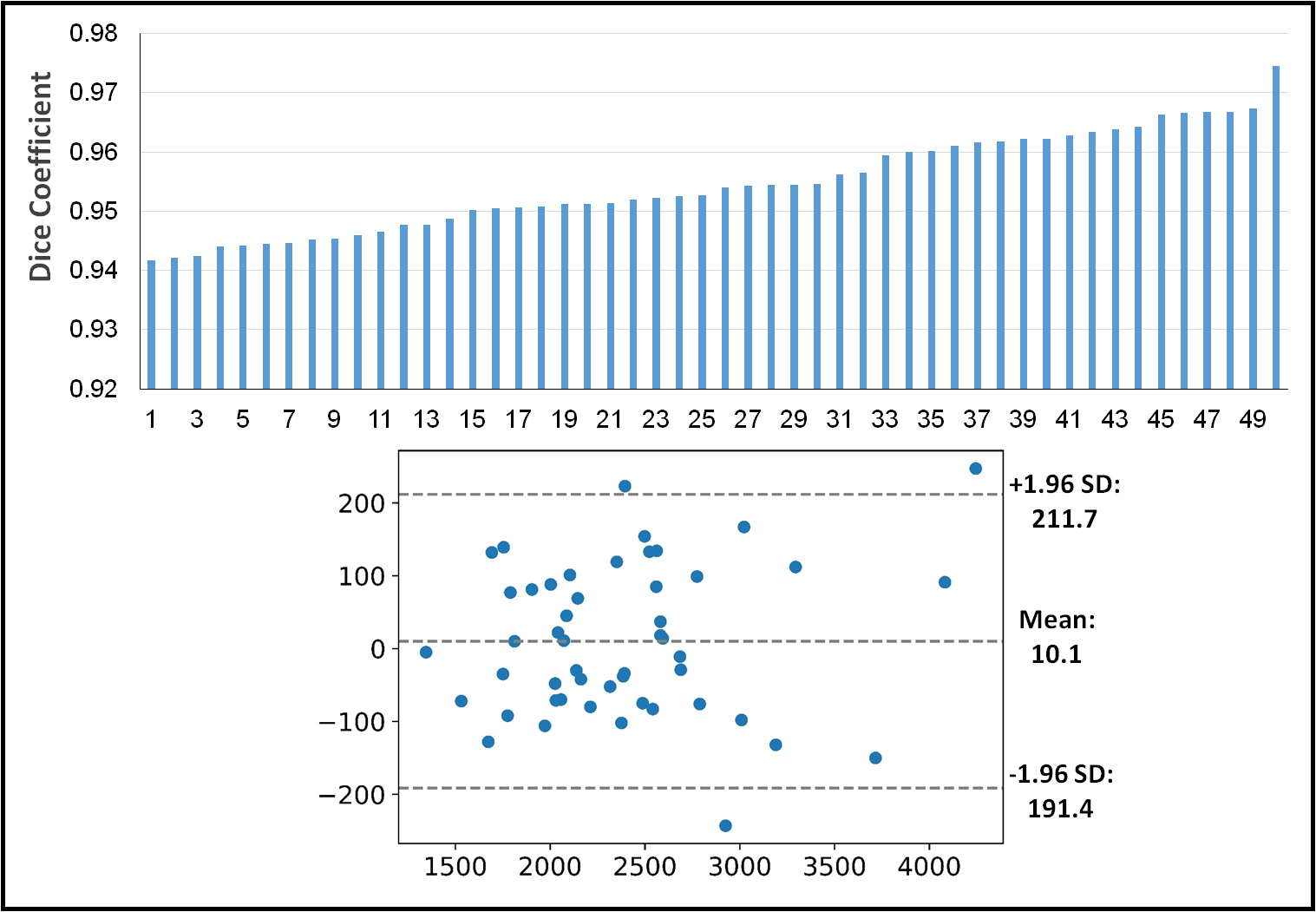
Top: the Dice
coefficient for all the livers in the test data set sorted from smallest to
largest. Bottom: Bland-Altman plot showing negligible bias.
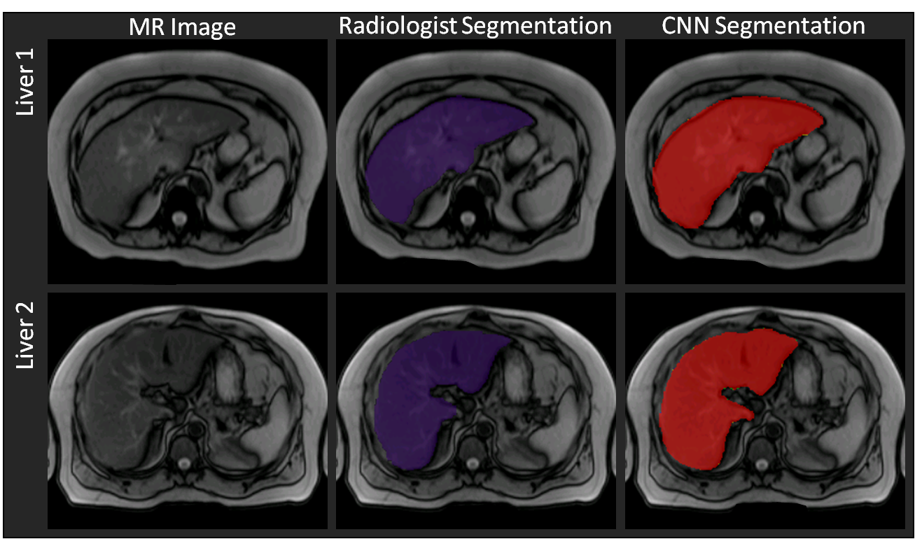
Comparison between
the radiologist’s manual segmentation (purple mask) and the automated CNN-based
segmentation (red mask). Good agreement
can be seen for the two livers between the manual and automated segmentations.