2728
Brain Segmentation in Rodent MR-Images Using Convolutional Neural Networks1Center for translational neuromedicine, University of Copenhagen, Copenhagen, Denmark, 2Department of Computer Science, University of Copenhagen, Copenhagen, Denmark, 3Department of Anesthesiology, Yale School of Medicine, New Haven, CT, United States, 4Institut for Mikro- og Nanoteknologi, Technical University of Denmark, Kgs. Lyngby, Denmark, 5Department of Neurosurgery, University of Rochester, Rochester, NY, United States
Synopsis
This study compares two different methods for the task of brain segmentation in rodent MR-images, a convolutional neural network (CNN) and majority voting of a registration based atlas (RBA) , and how limited training data affect their performance. The CNN was implemented in Tensorflow.
The RBA performs better on average when using a training set with fewer than 20 images but the CNN achieves a higher median dice-score with a training set of 19 images.
Introduction
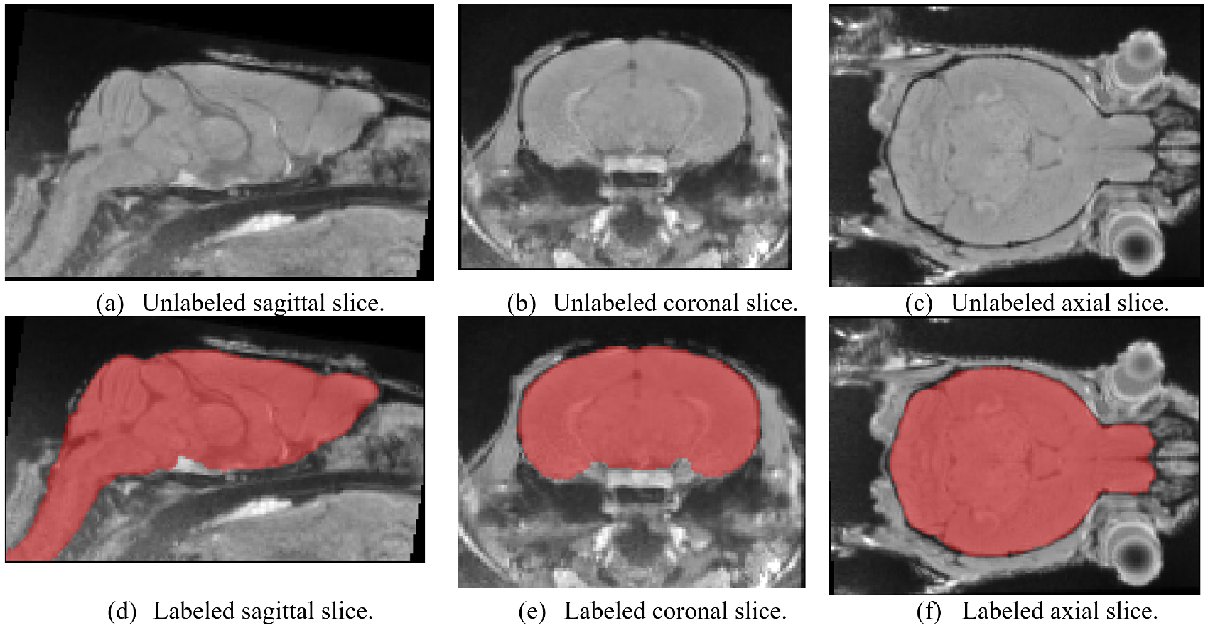
We present a study of the feasibility and practicality of using convolutional neural networks (CNN) to produce a brain segmentation of rodent MR-images (Fig. 1) compared to a registration based approach and how limited training data affect the performance of CNNs and registration. Rodents are widely used in experiments and manual segmentation of rodent MR-images is time-consuming, requires intimate knowledge of rodent anatomy and is subject to variability between image analysts. Automatic image segmentation provides faster and reproducible results. CNNs are a type of artificial neural networks that are well suited for processing images.1,2 CNNs have seen great success recently in performing a wide variety of image-related tasks.1Methods
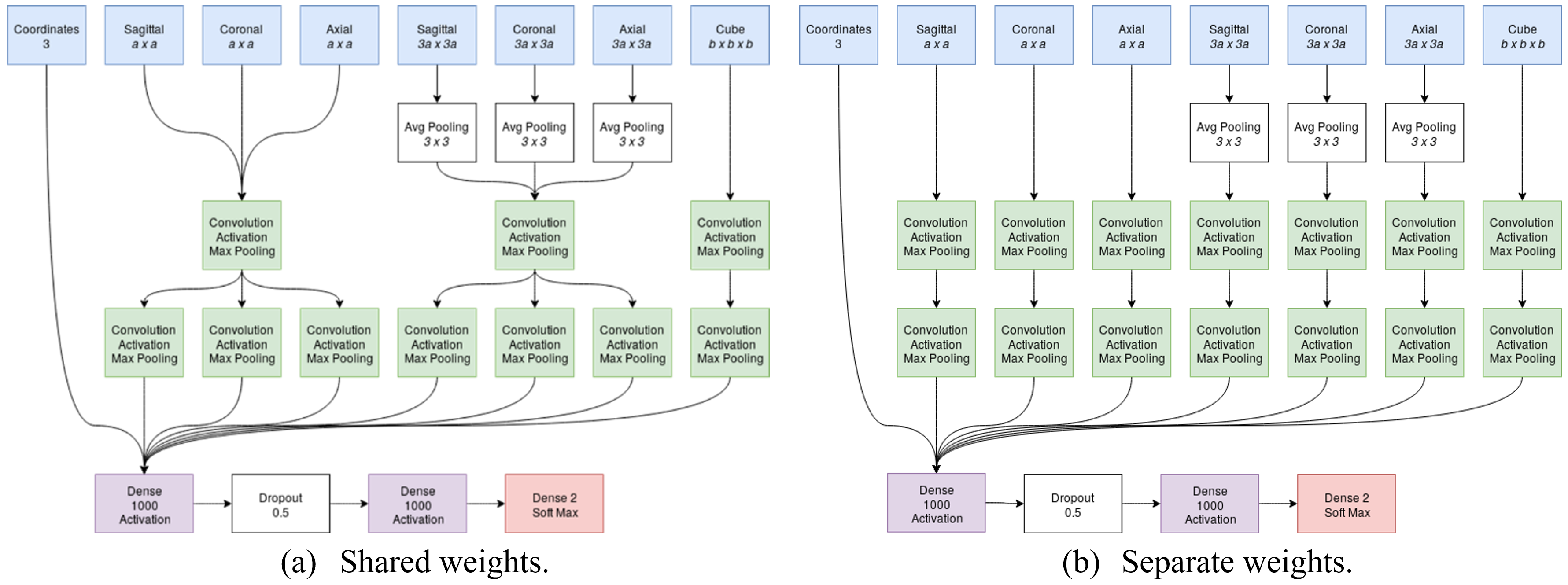
T1-weighted head images of mice were acquired on a Bruker BioSpec 9.4/30 USR scanner interfaced with an AVANCE III console controlled by Paravision 5.1 software, using a volume transmit coil and a surface quadrature receive coil, and consisted of a FLASH3D sequence (echo time: 4.425 ms, repetition time: 15 ms, flip angle: 15°, field of view: 2x1.5x1.5 cm3, matrix size: 160x120x120, isotropic resolution: 0.125 mm, 3 repetitions). A CNN designed for the purpose of brain-segmentation was implemented and tested on the MR-images. Segmentation using majority voting of a registration-based atlas (RBA) created with non-linear registrations was used for comparison. The images were bias-field corrected, motion corrected, and rigidly registered to a common baseline before training and testing. The CNN was trained on increasing number of manually segmented images and tested on a separate testing set. Cross-validation was used to produce results from multiple different training and testing sets. The CNN was implemented in Python using Tensorflow.3 ANTs was used for registrations.4 The design of the convolutional neural-networks is based on the work of the paper Deep Neural Networks for Anatomical Brain Segmentation from 2015.5 This design classifies every pixel in an image individually using 2D patches extracted from the axial, sagittal, and coronal planes of the image at two different scales. A 3D cube around the pixel of interest and its coordinates are also used as input features.Results
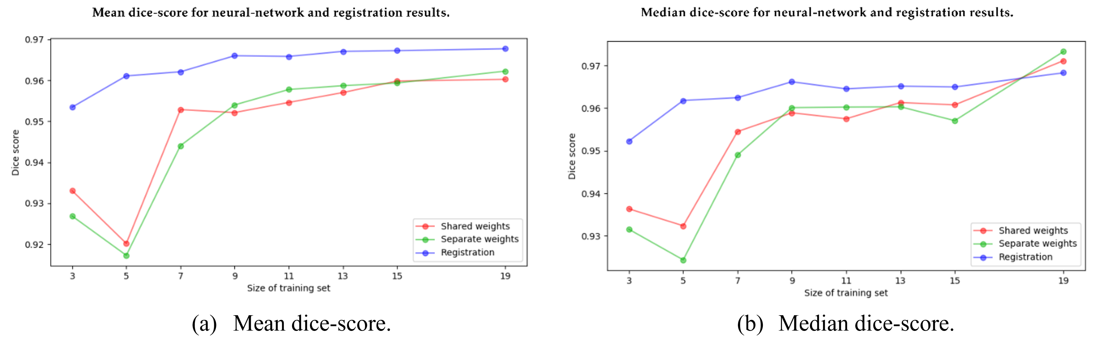
The resulting segmentations were evaluated using the dice-score between automatically and manually segmented images. On average, the CNN performed worse than the RBA (Fig 2a), although the median dice-score of CNN segmented images was higher than the median dice-score of RBA segmented images when training with 19 images (Fig 3b). Increasing the number of training images improved the performance of both CNN and RBA although the improvements were more dramatic for the CNN. Training with 11 images produced far better results than training it with 5 images. Training with 19 images marginally improved the results over 11 training images (Fig. 3).Discussion
The CNN performs comparably but slightly worse on average than the RBA when trained with 19 images and often produce a label with a higher dice score. The mean dice score is affected by several very poorly segmented images. The median dice score is higher for the CNN than the RBA but the mean score of the CNN is lower than the RBA when training with 19 images (Fig. 3b). This suggests that the CNN often produces a label with a higher dice-score than the RBA but sometimes produces a label with a much lower dice-score. The RBA consistently produces decent results even for poor quality images. Increasing the amount of training data improves the results swiftly for both the CNN and the RBA at first but the improvements plateau relatively quickly, at around 9 or 11 training images. The performance appears to continue to improve slowly past the 19 training images tested here (Fig. 3). A more complex CNN may be able use the images more effectively to achieve better results when training with more than 11 images.Conclusion
Segmenting rodent MR-images using CNNs is feasible and practical. The RBA produces better results on average than the CNN with a training set of fewer than 20 images but with a larger training set the CNN is likely to improve beyond the performance of the RBA. Good performance can be achieved using only a few labeled images to train on compared to the vast amounts of data often needed by traditional neural networks.2 Performing more experiments using different designs of the CNN and other data-sets would provide a better understanding of how well this method generalizes.Acknowledgements
This work was supported with grants from SVD@target and Foundation Leducq.References
1. Krizhevsky, A., Sutskever, I., & Hinton, G. E. (2012). Imagenet classification with deep convolutional neural networks. In Advances in neural information processing systems (pp. 1097-1105).
2. Glorot, X. & Bengio, Y.. (2010). Understanding the difficulty of training deep feedforward neural networks. Proceedings of the Thirteenth International Conference on Artificial Intelligence and Statistics, in PMLR 9:249-256
3. Abadi, M., Agarwal, A., Barham, P., Brevdo, E., Chen, Z., Citro, C., ... & Ghemawat, S. (2016). Tensorflow: Large-scale machine learning on heterogeneous distributed systems. arXiv preprint arXiv:1603.04467.
4. Avants, B. B., Tustison, N. J., Song, G., Cook, P. A., Klein, A., & Gee, J. C. (2011). A reproducible evaluation of ANTs similarity metric performance in brain image registration. Neuroimage, 54(3), 2033-2044.
5. de Brebisson, A., & Montana, G. (2015). Deep neural networks for anatomical brain segmentation. In Proceedings of the IEEE Conference on Computer Vision and Pattern Recognition Workshops (pp. 20-28).
Figures