Synopsis

Synthetic CT (sCT) must be generated directly from MRI scans to achieve MRI-only radiotherapy. We propose 2D and 3D convolution neural network models for generating pelvic sCT and evaluate their performance. Five-fold cross-validation is performed using paired T1-weighted MRI and CT scans from 20 patients. Our results show the 2D model generates accurate sCT for all patients in this study. The average mean absolute error (MAE) between CT and sCT across all patients is 38.0±3.9 HU in the 2D model. The average MAE is 55.9±28.4 HU in the 3D model. This large variation is possibly due to the limited number of 3D training volumes.

Introduction

Materials and methods

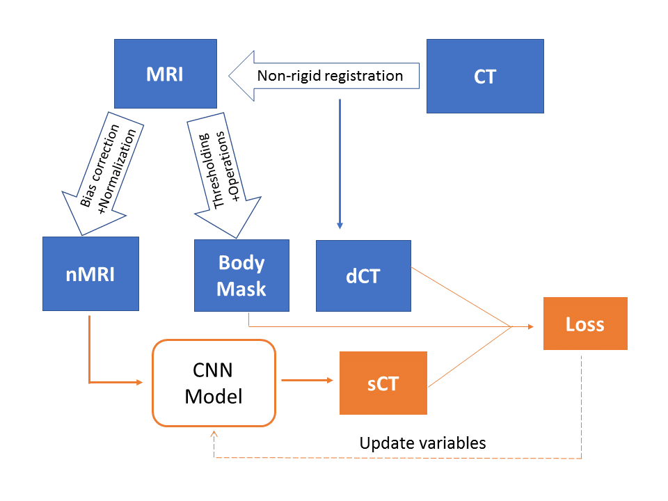
The overall workflow of sCT generation is shown in Figure 1. The T1-weighted MRI and CT scans of 20 prostate RT patients are retrospectively acquired. Thirty slices covering the pelvis are extracted from MRI scans and resampled to 256 × 256 ×30. The CT is registered to MRI using a multi-resolution B-spline algorithm in Elastix⁶. N4 bias filed correction⁷ and histogram-based normalization⁸ are performed on all MRI scans to ensure consistent MRI intensity throughout patients. A body mask of each patient, which is used to restrict loss evaluation and sCT accuracy assessment, is also generated from the MRI scan using Otsu's thresholding and morphological operations.

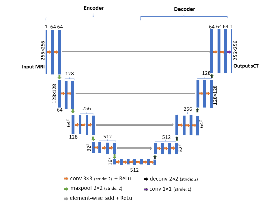
Our 2D and 3D CNN models are modified from SegNet⁵, a state-of-art deep learning architecture for semantic segmentation. First, de-convolution layers are used to replace upsampling layer to save computational memory. Second, residual shortcuts, connecting the encoder and decoder part, are added for faster convergence. Figure 2 shows the network architecture of the 2D model. The 3D model shares the same architecture except (1) all 2D operations are replaced with their 3D counterparts (2) a batch normalization layer is added after each 3×3×3 convolution layer for speeding up the training.

Both models are implemented using Tensorflow⁹ packages. On-the-fly data augmentation, such as random shift and rotation, is performed to reduce overfitting. The loss function is defined as mean absolute error (MAE) between sCT and deformed CT (dCT) within the body mask plus an L2 regularization term, i.e. $$loss=\frac{1}{N} \sum_{i=1}^{n}||sCT(i)-dCT(i)||+\lambda\sum_{i=1}^{k}ω_i^2$$

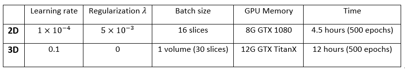
which is minimized using Adam stochastic gradient descent method with default parameters except for initial learning rate.¹⁰ Since the convolution layers of the VGG16 network¹¹ is identical to the encoder part of the 2D model, we initialize the weights of 2D encoder part using pre-trained VGG16 weights. All other weights of convolution filters are initialized using Xavier initialization12, and all bias parameters are initialized to 0. The details of training for two models are summarized in Figure 3.

Results

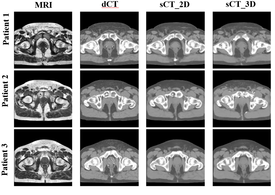
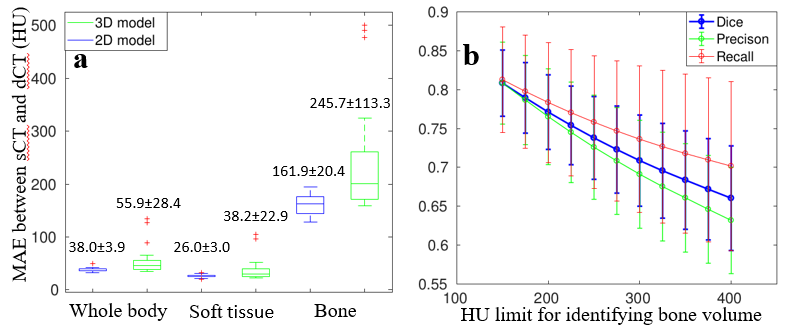
The sCT of every patient is generated in five-fold cross-validation framework. It only takes about 4 seconds to produce a sCT volume. Figure 4 shows three patients' sCT images with corresponding MRI-dCT image pairs. The 2D and 3D model generates sCT images which look similar to dCT images. However, the 3D model is not robust as shown in Figure 5a, the box-whisker plot of the MAE for different tissues across all patients. Cortical bone is mapped to soft tissue in 3D sCT for three patients as indicated in red cross above bone boxes of the 3D model.

Besides voxel-wise accuracy, as shown in Figure 5b we also present the dice similarity coefficient ($$$ \frac{TP}{2TP+FP+FN} $$$), recall ($$$ \frac{TP}{TP+FN} $$$) and precision( $$$ \frac{TP}{TP+FP} $$$) of bone volumes, which are defined using different HU thresholds, between dCT and sCT generated in the 2D model.

Discussion and conclusion

Acknowledgements

References