2717
Segmentation of Bone Tumor with MR imaging using Machine Learning1Centre for Biomedical Engineering, Indian Institute of Technology Delhi, New Delhi, India, 2Department of Computer Science and Engineering, Indian Institute of Technology Delhi, New Delhi, India, 3Department of Radiology, All India Institute of Medical Sciences, New Delhi, India, 4Department of Medical Oncology, IRCH, All India Institute of Medical Sciences, New Delhi, India
Synopsis
There has been a lot of work in segmentation of tumors in organs like the brain. Segmentation of bone tumor with MRI is not widely studied. Manual segmentation can be costly and time consuming. We study three automatic 3D segmentation techniques: Energy-based graph cuts, deep feed forward neural networks and mean shift clustering. Results show that, these methods can perform good quality segmentation (dice coefficient >70%) even with no human intervention. Tumor ADC values computed using these methods are comparable with those obtained from manual segmentation, showing that these methods can be used as a screening tool.
Introduction:
Segmentation is the first step in developing a pipeline for automated image analysis (like perfusion and diffusion analysis) of bone tumor. Moreover, bone tumor segmentation is challenging due to high variability in shape/structure across different types of bones1. Manual segmentation is time consuming and has high inter- and intra-rater variability2. It is thus important to investigate automated segmentation techniques that work well without requiring much human intervention.Methods:
MRI dataset of twenty (M:F=16:4, 15.5±2.6yrs) patients with osteosarcoma was acquired under the Institutional protocol (IEC-103/05.02.2016,RP-26/2016). Acquisition was performed using 1.5T Phillips Acheiva MRI scanner. T1 and T2 images were acquired using TSE sequence with TR/TE=644/10 and 73795/85, matrix size=512×512 and 384×384 respectively. DWI was acquired using Spin Echo-Echo Planar Imaging (SP-EPI) with TR/TE=7541/67msec, matrix size=192×192, slice thickness/Gap=5mm/0.5mm, voxel size=2.98/3.52/5.0mm, b-values=0-800s/mm2 and 64 axial slices. Three techniques were implemented for bone tumor segmentation. These techniques have been successfully used in lung and brain tumor segmentation3,4,5,6.
1) Energy-based graph cut7: Each node in the graph corresponds to a voxel in DW image, and must be labeled as either tumor or non-tumor. Regional cost Rp and neighborhood cost Bpq are assigned and total cost C=Rp+Bpq is minimized using a min-cut algorithm. Regional cost can be assigned in two ways that gives two algorithms:
a. T-GC: Uses Thresholding on intensity values in DW image
b. LR-GC: Uses prior probability from Logistic Regression
2) Deep feedforward neural network (DNN)8: Prediction is made for each voxel independently whether or not belonging to bone. 15 textural features per modality (DWI with b=800s/mm2, T1, T2 and PDW) are generated using gray-level co-occurrence matrix (GLCM) and gray-level run length matrix (GLRLM)1,9. The network has two hidden layers with 64 units each and rectified linear unit (ReLU) non-linearity, and an output layer of 1 unit with sigmoid non-linearity to generate a probability value. 10% of the data is used as validation set and early stopping is used to prevent overfitting.
3) Mean shift clustering10 (MSC): This technique divides the 3D DW image into density-based clusters and automatically decides the number of clusters in the image. The only human input required is in the last stage deciding which cluster is the predicted tumor.
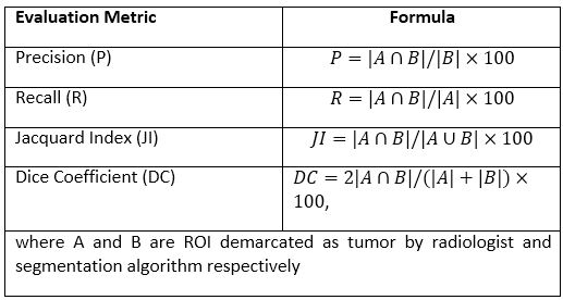
Ground truth tumor ROIs marked by a radiologist (>9 years experience in cancer imaging) were used for evaluation. Evaluation metrics used are precision(P), recall(R), dice coefficient(DC) and jacquard index(JI) as elaborated in table1. Otsu-thresholding11 is reported as a baseline segmentation method for comparison. Four-fold cross validation was performed for all data-driven methods. Mean ADC value for tumor ROI across patients using different segmentation algorithms was calculated for comparison. Feature generation, graph cut and MSC were implemented in MATLAB-R2016B. DNN was implemented in python using Keras.
Results:
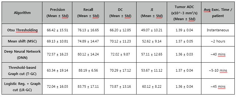
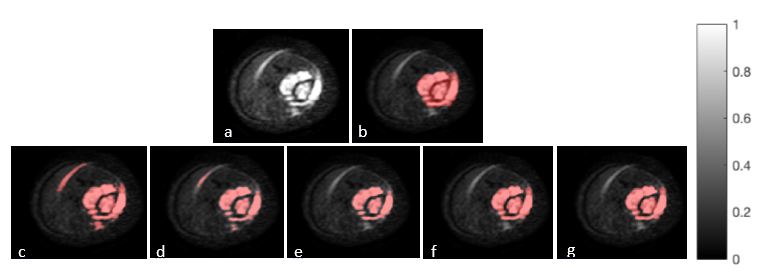
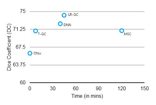
Table2 shows the metrics of performance, execution time and average ADC value for tumor mask for each segmentation algorithm. LR-GC showed good segmentation wuth DC~74±13%, followed by DNNs (DC~72±10%). MSC (DC~70±11%) and T-GC (DC~70±17%) showed similar performance. All segmentation algorithms performed better than simple Otsu-thresholding. T-GC is the fastest (~5-10 mins) while MSC takes ~2 hours. The best performing method, LR-GC, had tumor ADC of 1.36±0.04x10⁻³mm2/s which is comparable to ADC values calculated with tumor mask by radiologist 1.33±0.03x10⁻³mm2/s. Figure1 shows segmentation results from different algorithms for a representative patient. Figure2 shows the DC vs computation time for five segmentation methods.Discussion:
LR-GC gives better performance because logistic regression can make use of textural features and weights learnt from data to generate good probabilities, and graph cut uses neighborhood structure to refine the predictions from logistic regression and give a coherent prediction. DNNs can learn complex non-linear functions of the input features and using recently introduced regularization techniques like early stopping helps in generalizing to test data. T-GC is fast but has lower precision and high recall, so it segmented most of the tumor region but may also has false positives. This is because it uses just intensity values without exploiting information from data. MSC is comparatively slow because it has a time complexity of O(n2). Thus, for new data, T-GC can be used if high speed is needed or training data is unavailable, but otherwise DNNs or LR-GC is recommended. Mean ADC for gold mask and mask given by these techniques are comparable which means these techniques can be used as screening tools.Conclusion:
We show that fully automated bone tumor segmentation techniques provide good quality segmentation. They can significantly reduce human effort and can help enable a pipeline for automated image analysis.Acknowledgements
Authors would like to thank staff at All India Institute of Medical Sciences, New Delhi for helping patient recruitment and providing clinical support.References
1. Mehndiratta et. al., Textural Analysis based Segmentation of Bone Tumors using Diffusion weighted MR image, Proc. 25th ISMRM, 2017 2. Collier et. al., Assessment of consistency in contouring of normal-tissue anatomic structures, JAPCM, vol. 4, no. 1, pp. 17–24, 2003. 3. Birkbeck et al., An interactive graph cut method for brain tumor segmentation, WACV, pp. 1-7, IEEE, 2009. 4. Ballangan et al., Lung tumor segmentation in PET images using graph cuts, Comp. Meth. Prog. Biomed., 109.3: pp. 260-268, 2013 5. Mayer and Greenspan, Segmentation of brain MRI by adaptive mean-shift, Int. Symp. Biomed. Imag. (ISBI), 2006, pp. 319-322 6. Havaei et al., Brain tumor segmentation with deep neural networks., Medical image analysis, 35 (2017): pp. 18-31. 7. Boykov and Funka-Lea, Graph Cuts and Efficient N-D Image Segmentation, IJCV, 70 (2), pp. 109-131, 2006 8. Goodfellow et. al., Deep learning, MIT Press, 2016 9. Haralick et. al., Textural Features for Image Classification, IEEE Trans. Sys., Man., Cyber, vol. SMC-3, pp. 610-621, 1973 10. Comaniciu and Meer, Mean shift: a robust approach toward feature space analysis, IEEE Trans. Patt. Anal., Mach. Int., 24(5):pp. 603-619, 2002 11. Noboyuki Otsu, A threshold selection method from gray-level histograms, IEEE Trans. Sys., Man., Cyber., 9(1): pp. 62-66, 1979Figures