Synopsis

We developed 3D Cones sequences for human extremities on a 1.5 T MRI system using a compact superconducting magnet (280 mm bore) equipped with an unshielded gradient coil. Linear eddy fields were measured using a spherical phantom and eddy current effects on the 3D Cones sequences were evaluated using a 3D water phantom. As a result, effects of higher-order eddy fields proportional to z²x and z²y spatial distributions were clearly observed. The 3D Cones sequences were applied to UTE imaging of a porcine hoof sample and a human forearm, which demonstrated their promise in UTE imaging.

Introduction

Materials and Methods

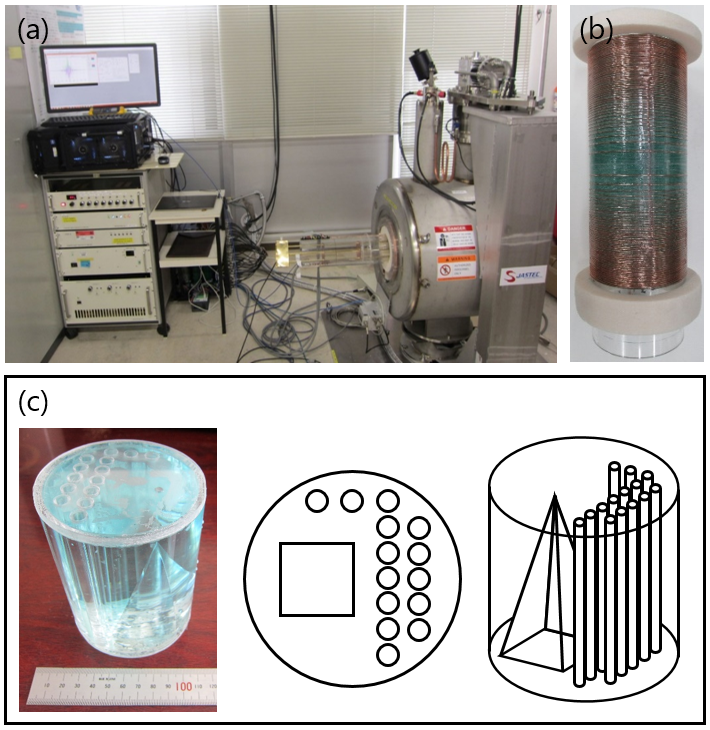
Figure 1(a) shows an overview of the home-built compact MRI system using a 1.5T horizontal bore (280 mm) superconducting magnet (JASTEC, Kobe, Japan) used in this study. This system is controlled by a fully-digital MRI console (DTRX6, MRTechnology, Tsukuba, Japan). Figure 1(b) shows an unshielded gradient coil set (inner diameter = 160mm). 3D Cones sequence was designed after Glover [1]. Figure 1(c) shows a 3D water phantom used for evaluation of the 3D Cones sequence.

Linear eddy fields caused by switching of the gradient coil currents were measured using spherical CuSO₄ aqueous solution stored in a plastic sphere (inner diameter=23.5 mm). The linear eddy fields were analyzed by temporal shifts of the gradient-echo peak measured for gradient pulses with variable delay times (delay time = 0.01 to 100 ms) applied before the RF excitation pulse. The 3D Cones imaging was performed for the 3D water phantom, porcine hoof sample, and human forearm. For comparison, conventional gradient-echo imaging was performed for these objects.

Results

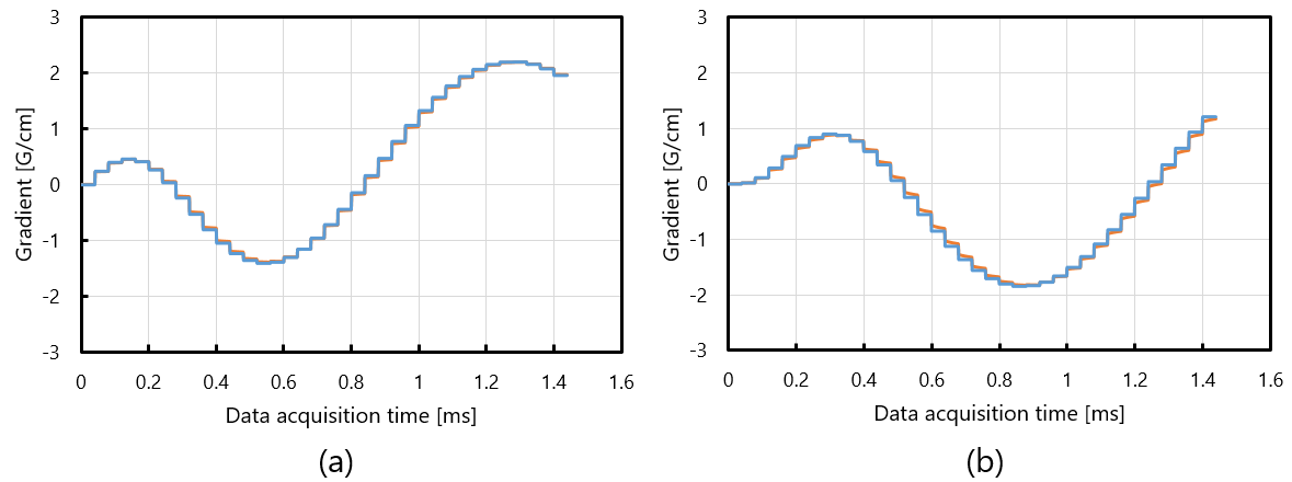
The linear eddy fields observed for the various delay times were decomposed to two exponentially decaying components with different amplitudes and time constants. The combination of the relative amplitudes (induced linear eddy field / applied gradient field) and the time constants of the linear eddy fields caused by Gx were (6.4%, 0.077ms) and (0.57%, 23.4ms), and those by Gy were (19%, 0.046ms) and (0.60%, 23.4ms), respectively. Figure 2(a) and (b) show estimated gradient fields with (orange) and without (blue) the linear eddy fields for (a) Gx and (b) Gy gradients. These figures demonstrate that the gradient waveforms are slightly delayed by the linear eddy fields.

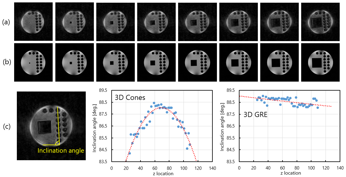
Figure 3(a) and (b) shows axial cross-sections selected from 3D image datasets of the 3D water phantom acquired with (a) the 3D Cones and (b) the conventional 3D gradient-echo sequences. Figure 3(c) shows the inclination angle of the central line of the acrylic rods in the axial images plotted against the z for the 3D Cones and the conventional gradient-echo sequences. These graphs clearly show that the axial images acquired with the 3D Cones rotate proportional to (z-z₀)², where z₀ is the central coordinate along the axial position.

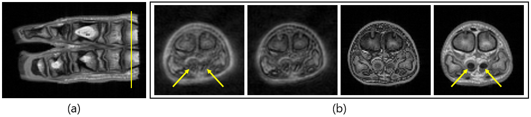
Figure 4(a) shows a coronal cross-section of the porcine hoof sample acquired with a conventional gradient-echo sequence (TR=200ms, TE=4.6ms). Figure 4(b) shows axial cross-sections at the yellow line shown in Fig.4(a) acquired with 3D Cones (TE=0.4ms and 1.0ms) and conventional 3D gradient-echo (TE=2.3ms and 4.6ms) sequences. Image intensities lost in the 3D GRE image (TE=4.6ms) at deep flexor tendons recovered in the 3D Cones image (TE=0.4ms) as shown by the yellow arrows.

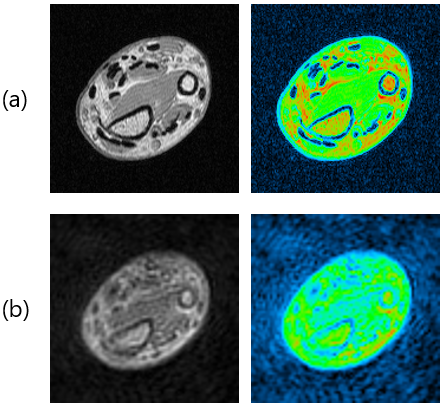
Figure 5 shows cross-sectional images selected from a 3D image dataset of a human forearm acquired with (a) a conventional 3D gradient-echo sequence (TE=4.6ms) and (b) the 3D Cones sequence (TE=0.4ms). Image intensities lost in the 3D GRE image at tendons slightly recovered in the 3D Cones image.

Discussion

The change of the inclination angle along the z direction observed for the GRE axial images (Fig.3(c)) includes imperfections of the 3D water phantom and the gradient coil, and errors in the phantom setting. On the other hand, the change of the inclination angle observed for the 3D Cones axial images shows a clear parabolic change, which suggests presence of eddy fields proportional to z²x or z²y. This is because linear eddy fields cause delay of the gradient waveform as shown in Fig.2. Because the angular velocity of the k-trajectory of the 3D Cones sequence (64 shot) is about 2π/1.4ms or about 1.3 degree/(5 µs), about 4 degree difference between the central and the end of the axial images corresponds to about 15 µs delay of the gradient waveform at the end of the axial plane. Therefore, the axial image rotation of the 3D Cones image should be corrected to obtain geometrically correct MR images.

In conclusion, 3D Cones sequences were successfully implemented on our compact 1.5T MRI system and demonstrated their usefulness for the 3D UTE imaging.

Acknowledgements

References