Synopsis

Field maps are essential in spectroscopy, shimming, MR thermometry and geometric distortion correction. Minimizing the noise in acquired field maps is therefore potentially important to all of these applications. When using a multi-gradient echo, the choice of echo times has a marked effect on the noise on the acquired field maps. Here, we derive the optimal echo times which minimize the amount of noise in the resulting field maps.

Introduction

Theory

The problem of estimating $\Delta \nu$ from N phases $\phi_j=2\pi \cdot \Delta \nu \cdot TE_j + \phi_0$ (j=1,...,N) can be formulated using least squares: Ax=p, where $\mathbf{x}^T = \left( \Delta \nu, \Delta \phi \right)$, $\mathbf{p}^T = \left(\phi_1, \phi_2, ..., \phi_N \right)$ and a matrix A such that $A_{i,1}=TE_i$, $A_{i,2}=1$. The estimator for x is then $\mathbf{\hat{x}}=(A^T V^{-1} A)^{-1} A^T V^{-1} \mathbf{p}$, where V is the covariance matrix of the phases, $V_{ij}=Cov(\phi_i,\phi_j)$. V can be derived from the SNR in the magnitude image (SNR₀) [5], and can be shown to equal $V_{ij}=\delta_{ij}\frac{exp^{2TE_j/T_2^*}}{2SNR_0^2}$. Using that,

$$\Delta\hat{\nu}=\frac{1}{2\pi T_2^*}\cdot\frac{cov_w(x,\phi)}{var_w(x)}$$

where $x_j\equiv TE_j/T_2^*$, $w_j\equiv\exp(-2x_j)$, and $T_2^*$ is assumed known. The weighted variance and covariance are $var_w(x)=\left<x^2\right>_w-\left<x\right>_w^2$, $cov_w(x,\phi)=\left<x\cdot\phi\right>_w - \left<x\right>_w\left<\phi\right>_w$ with the weighted average of any quantity x defined as $\left<x\right>_w \equiv \frac{\sum_{j=1}^N w_jx_j}{\sum_{j=1}^N w_j}$.

The covariance matrix of the least squares estimator is given by $V_{\mathbf{\hat{x}}}=\left(A^TV^{-1}A\right)^{-1}$, under the assumption that A contains no uncertainty, which is valid in our case. Explicitly evaluating $V_{\mathbf{\hat{x}}}$ then provides us with a closed form expression for the variance of the frequency estimator $\Delta\hat{\nu}$:

$$\sigma_{\Delta\hat{\nu}}=\frac{1}{2\pi\sqrt{2}SNR_0T_2^*}\sqrt{\frac{1}{\left(\sum_{j=1}^N w_j \right)\cdot var_w(x)}} \equiv \frac{f(x_1,x_2,...,x_N)}{2\pi\sqrt{2}SNR_0T_2^*}$$

This error (in Hz) in the field map is SNR-dependent and therefore varies from voxel to voxel.

Methods

Numerical Optimization: To minimize the error in the field maps, $\sigma_{\Delta\hat{\nu}}$, we solved a nonlinear constrained minimization problem using standard interior point methods in MATLAB (The Mathworks, Natick, MA): $\min_{x_1,x_2,...,x_N} f(x_1,x_2,...,x_N)$ subject to $0\leq x_j \leq 5$, $x_j+\delta \leq x_{j+1}$, $x_1=0$.

Phantom Experiments: : We compared the calculated and experimental noise in a spherical 8 cm radius homogeneous water phantom doped with 1.5 mM Gd, to ensure a spatially homogeneous $T_2=T_2^*$. A multi-echo sequence ($TE_j=3,10,25,40$ ms, slice thickness = 2 mm, TR=1000 ms, TA=1:42 min, 35 slices, in plane FOV=256×256 mm2, matrix: 128×128) was first used to estimate T₂ in each voxel using an exponential fit of the magnitude images. Based on T2, a double gradient echo with optimal TE was run with the optimal echo times found during the Numerical Optimization. The noise’s standard deviation in the field map (following 4th order polynomial detrending) was estimated in a spherical subregion and compared to the theoretical prediction of $\sigma_{\Delta\hat{\nu}}$.

Results

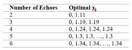
Numerical optimization: Table 1 shows the optimal echo times for N=2,3,…,6 echoes for the case of no minimial echo spacing ($\delta=0$). While $TE_1=0$, latter echoes assume identical values. The $\delta>0$ cases (not shown) merely spread the latter echoes tightly around this latter ($\delta=0$) value.

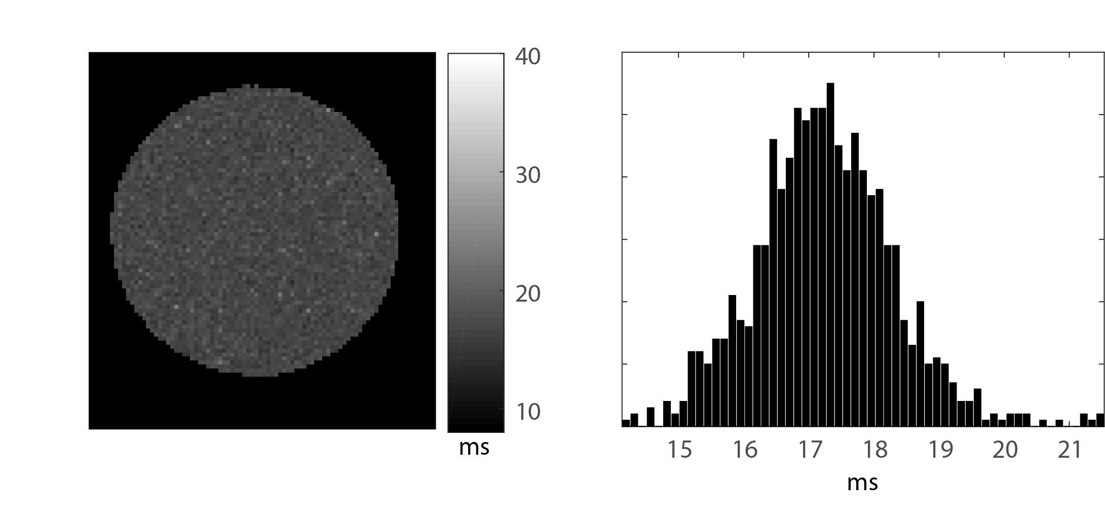
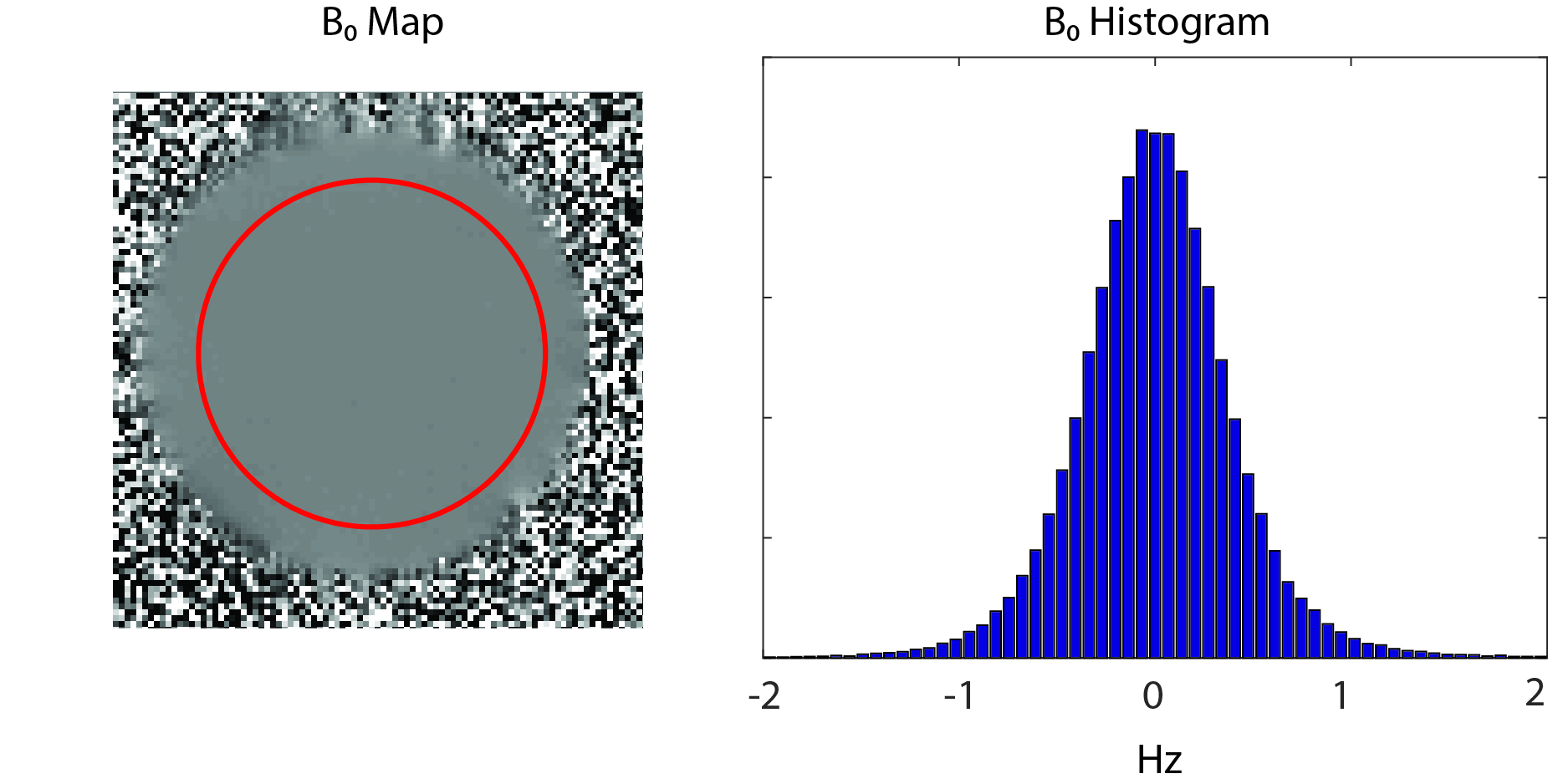
Phantom Experiments: Exponential fitting yielded a homogeneous distribution of T2 values within the GRE voxels of T₂=16.6±0.9 ms (Fig. 2).This is the true T2 of the sample, as further verified independently using single voxel variable TE MRS (not shown). According to Table 1, the optimal echo times are to be placed at the minimal TE, $TE_1=3$ ms for our sequence, $TE_2=TE_1+1.11\cdot T_2=21.4$ ms. Fig. 3 shows the distribution of B0 values obtained with the optimal echo times within a prescribed region, after detrending, with mean±s.d.=0.00±0.42 Hz. The theoretical prediction, for comparison, yields $\sigma_{\Delta\hat{\nu}}=0.39$ Hz, in excellent agreement. We've used a mean value for the magnitude image SNR within the prescribed region, which we measured to be $SNR_0\approx 53$. This validates our theoretical calculations.

Discussion & Conclusions

We've derived optimal echo times whichi minimize the noise in gradient echo based field maps. Intuitively, the timescales involved are on the order of $T_2^*$. Counter-intuitively, perhaps, is the distribution of echo times: a single echo is placed at TE=0, i.e., as early as possible, while remaining echoes are placed as close together around TE≈T2*.

We note the optimal echo times derived herein relate only to noise levels. They may not necessarily be optimal when considered, e.g., from the point of view of phase wrapping.

Acknowledgements

References

[1] Stockmann JP, Wald LL. In vivo B0 field shimming methods for MRI at 7T. Neuroimage 2017.

[2] Rieke V, Pauly KB. MR thermometry. Journal of Magnetic Resonance Imaging 2008;27(2):376-390.

[3] Pan JW, Lo KM, Hetherington HP. Role of very high order and degree B0 shimming for spectroscopic imaging of the human brain at 7 tesla. Magnetic resonance in medicine 2012;68(4):1007-1017.

[4] Jezzard P. Correction of geometric distortion in fMRI data. Neuroimage 2012;62(2):648-651.

[5] Gudbjartsson H, Patz S,The rician distribution of noisy mri data. Magn Reson Med 34:910-914 (1995)