Synopsis

A new form of B1-insensitive excitation is introduced, termed Spin-Lock Adiabatic Correction (SLAC) excitation, that combines a Spin-Locking excitation with an orthogonal Adiabatic Correction to more uniformly flip the magnetisation across a range of B1 strengths. SLAC pulses achieve adiabatic-like excitation, in terms of B1-insensitivity, in faster excitation time while not increasing the delivered power. We demonstrate the advantages of SLAC pulses in both simulation and phantom experiments. Decreasing the pulse duration causes performance breakdown of the adiabatic pulse due to violation of the adiabatic condition, while the SLAC pulse maintains control of magnetisation across the range of B1 strengths.

Introduction

The predominant causes of inhomogeneity in B1 excitation fields are hardware based, in the case of surface transmit coils, and tissue based, particularly prevalent in high field MRI systems¹. B1 inhomogeneity results in flip angle variation when using conventional RF pulses, which produces signal strength non-uniformity¹. Attempts to address B1 inhomogeneity include the use of parallel transmit systems², pulse design^3,4 and post-processing⁵ methods. A new class of B1-insensitive RF pulses, termed Spin-Lock with Adiabatic Correction (SLAC) pulses, is introduced that extends the utility of adiabatic pulses beyond the rate-limiting breakdown of the adiabatic condition, as demonstrated here in both simulation and experiment.

Theory

We first define an adiabatic half passage as follows. Consider a pulse of length $$$T_p$$$. Let $$$\Delta\omega_{0}^{max}$$$ be the maximum frequency sweep and $$$\omega_{1,max}$$$ be the maximum amplitude of an adiabatic half passage (AHP) defined by amplitude and phase functions:

$$\omega_{1}^{\textrm{AHP}}(t)=\omega_{1,max}\tanh\left(\frac{\zeta t}{T_p}\right)$$ $$\phi^{\textrm{AHP}}(t)=\int_0^t\Delta\omega_0(t^\prime) dt^\prime=-\frac{\Delta\omega_0^{max}T_p}{\kappa\tan\kappa}\left(\log\cos\kappa-\frac{1}{\cos\kappa}\log\cos\left(\kappa\left(1-\frac{t}{T_p}\right)\right)\right)$$ where $$ \Delta\omega_0(t)=\Delta\omega_0^{max}\frac{\tan\left(\kappa\left(1-\frac{t}{T_p}\right)\right)}{\tan\kappa}$$

Here $$$\kappa$$$ and $$$\zeta$$$ are AHP shape parameters⁶.

The resultant effective field angle is:

$$\alpha^{\textrm{AHP}}(t)=\arctan\left(\frac{\omega_{1}^{\textrm{AHP}}(t)}{\Delta\omega_0(t)}\right)$$

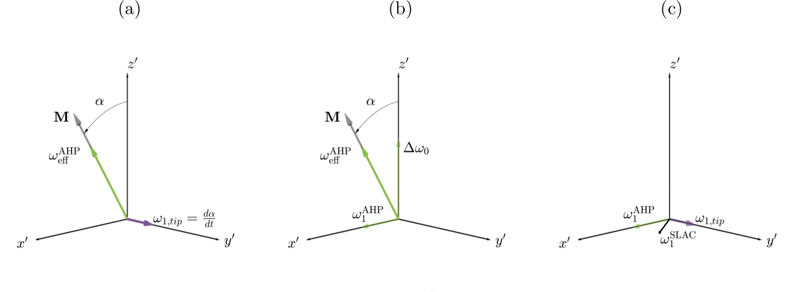
SLAC pulses combine an effective B1 field applied as a spin-lock along the direction of the bulk magnetisation, with a B1 field applied orthogonal to the bulk magnetisation, $$$\omega_{1,tip}$$$. The spin-locking component of the SLAC pulse is applied as an AHP such that $$$\omega_{eff}^{\textrm{AHP}}$$$ tracks the bulk magnetisation as it is tipped by the orthogonal component, $$$\omega_{1,tip}$$$ (Figure 1(a)).

The SLAC amplitude is a vector sum of the $$$\omega_{1}^{\textrm{AHP}}$$$ and $$$\omega_{1,tip}$$$ components, $$\omega^{\textrm{SLAC}}_1(t)=\sqrt{\omega_{1}^{\textrm{AHP}}(t)^2+\omega_{1,tip}(t)^2}$$ where $$$\omega_{1,tip}$$$ is the derivative of the AHP effective field angle, $$\omega_{1, tip}(t)=\frac{d\alpha^{\textrm{AHP}}(t)}{dt}\\\quad\quad\,\,\,= \frac{\frac{\omega_{1,max}\zeta \tan\kappa(\tanh\left(\frac{\zeta t}{T_p}\right)^2-1)}{\Delta\omega_0^{max}T_p\tan(\kappa(\frac{t}{T_p}-1))} +\frac{\kappa\omega_{1,max}\tanh\left(\frac{\zeta t}{T_p}\right)\tan\kappa\left(\tan(\kappa(\frac{t}{T_p}-1))^2+1\right)}{\Delta\omega_0^{max}T_p\tan(\kappa(\frac{t}{T_p}-1))^2}}{\left(\frac{\omega_{1,max}\tanh(\frac{\zeta t}{T_p})\tan\kappa}{\Delta\omega_0^{max}\tan(\kappa(\frac{t}{T_p}-1))}\right)^2+1}$$

The SLAC phase is a function of the $$$\phi^{\textrm{AHP}}$$$ and the ratio of the strengths of the $$$\omega_{1}^{\textrm{AHP}}$$$ and $$$\omega_{1,tip}$$$ components: $$ \phi^{\textrm{SLAC}}(t)=\phi^{\textrm{AHP}}(t)+\arctan\left(\frac{\omega_{1,tip}(t)}{\omega_{1}^{\textrm{AHP}}(t)}\right)$$

While $$$\alpha^{\textrm{AHP}}$$$ is small it is roughly proportional to $$$\omega_1$$$ amplitude, and magnetisation nutation due to $$$\omega_{1,tip}$$$ is proportional to $$$\omega_1$$$ amplitude. This results in bulk magnetisation remaining collinear with $$$\omega_{eff}^{\textrm{AHP}}$$$ despite variation in $$$\omega_1$$$ amplitude due to B1 inhomogeneity. As $$$\alpha^{\textrm{AHP}}$$$ increases, bulk magnetisation that experiences a B1 field that varies from the reference B1 strength no longer remains collinear with $$$\omega_{eff}^{\textrm{AHP}}$$$ and the spin-locking effect of $$$\omega_{eff}^{\textrm{AHP}}$$$ produces an adiabatic-type correction.

Method

In both simulation and experiment the SLAC and AHP were peak power matched.

Simulated data:

Numerical simulation of the Bloch equations was performed using MATLAB to demonstrate the behaviours generated by the SLAC pulses over a range of B1 field strengths. Simulations of power-matched AHP pulses were carried out for comparison. The pulse parameters were $$$\zeta$$$=20, $$$\kappa$$$=$$$\arctan(20)$$$, $$$\Delta\omega_{0,max}$$$=20kHz, $$$T_p$$$=500$$$\mu$$$s, $$$\omega_{1,max}$$$=1.12kHz, resulting in $$$\omega_{1,max}$$$ of 1kHz for the power-matched SLAC pulse.

Experimental data:

Experiments were performed on a Bruker 4.7T MRI using a test-tube of water doped with Magnevist at a concentration of 100units/L. Excitation pulses were applied using a Bruker Cryoprobe surface Tx/Rx coil, as this coil naturally exhibits a B1 field gradient, allowing investigation of the performance of the pulses across a range of B1 field intensities. A UTE3D sequence was used for k-space acquisition (TR=2000ms). Data was acquired using SLAC, AHP and 90 degree block pulses of duration $$$T_p$$$=500$$$\mu$$$s and $$$\omega_{1,max}$$$=1.12kHz $$$\Delta\omega_{0}^{max}$$$=20kHz.

Results and Discussion

Simulation:

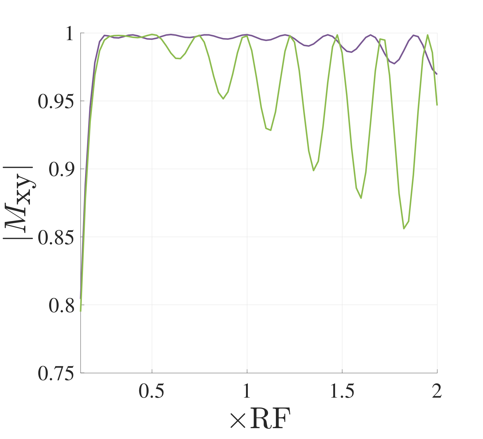
SLAC pulses extend the usable range of adiabatic pulses, as evidenced by the smaller fluctuation in transverse magnetisation over a range of B1 field strengths than an AHP pulse, when applied fast enough that the adiabatic condition breaks down for areas of higher B1 field strength (Figure 2). Note that this may seem counterintuitive, but for high B1 field strength the rate of change of the effective magnetisation is too rapid.

Experiment:

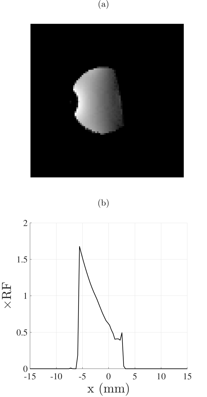
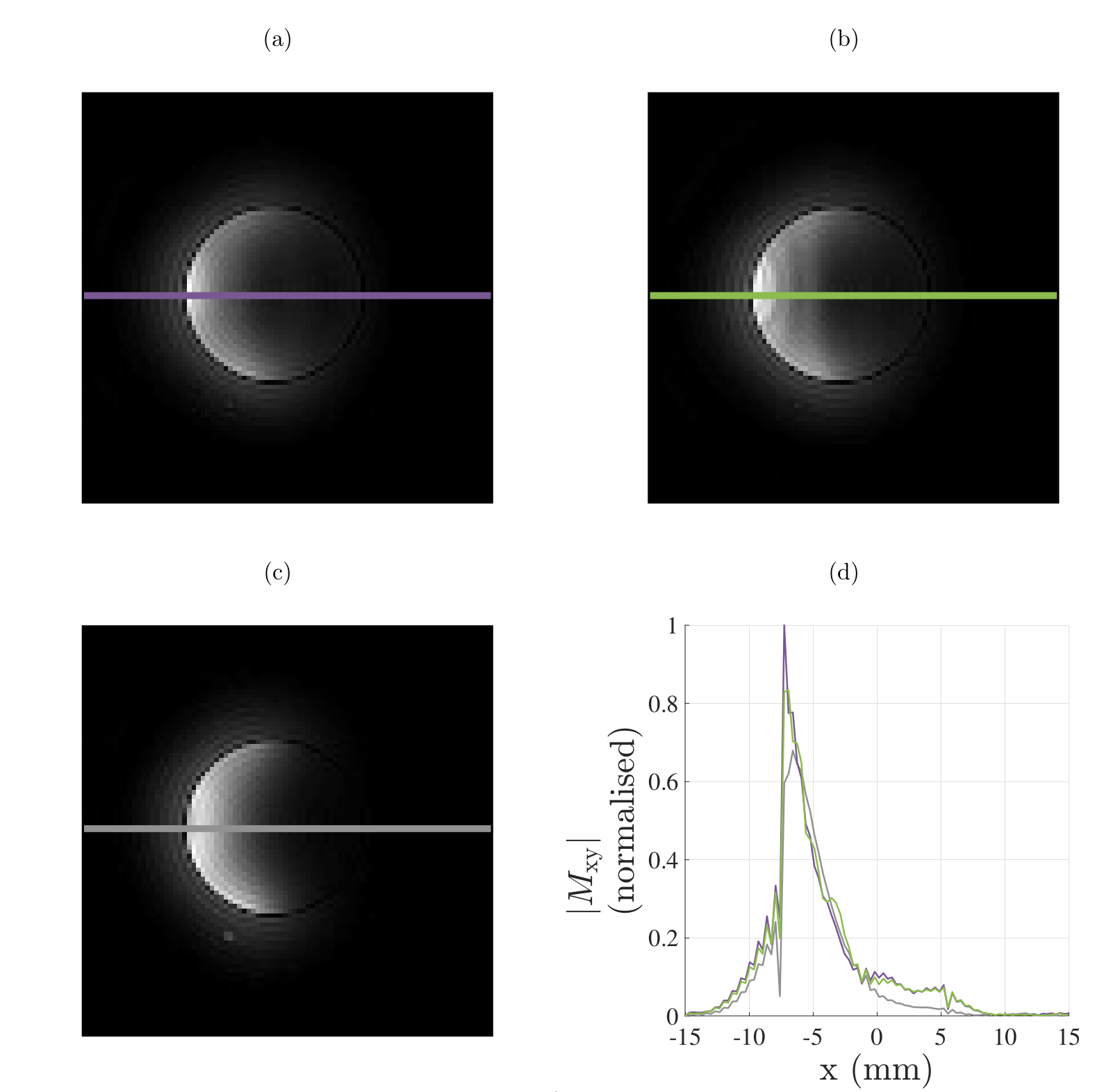
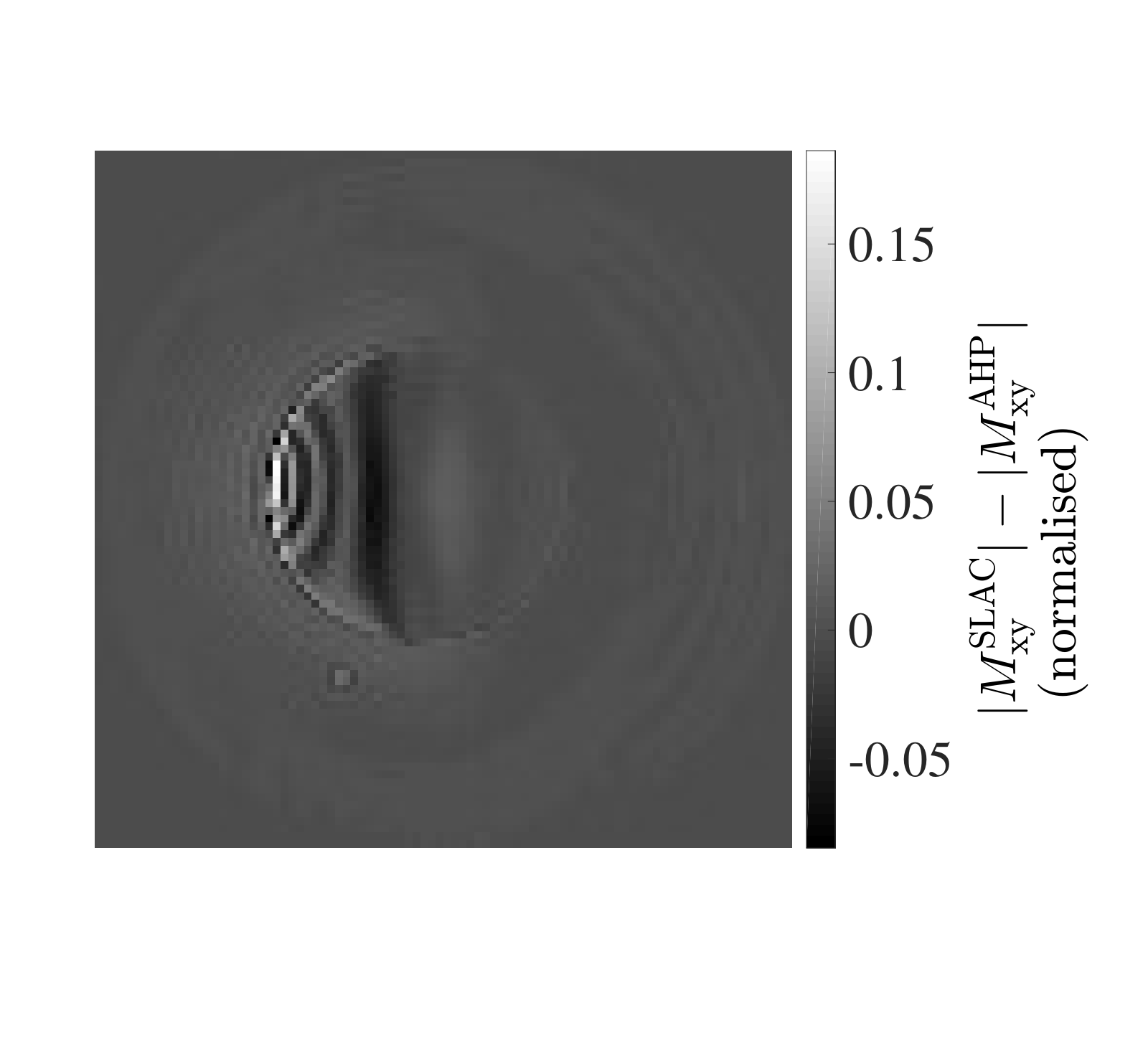
The experimental images acquired using a surface coil (B1 map in Figure 3) verify our simulation results, that when AHP pulses are driven quickly, they break down and produce fluctuation in the signal across B1 field strengths, as evidenced by the line profiles (Figure 4) and the difference image (Figure 5). The SLAC pulse mitigates this breakdown, achieving significantly less fluctuation across the wide range of B1 fields strengths representative of those encountered in high field MRI systems. The block pulse, as expected, gives a faster signal drop-off (Figure 4).

Conclusion

Acknowledgements

We acknowledge the facilities, and the scientific and technical assistance of the Australian National Imaging Facility at the Melbourne Brain Centre Imaging Unit. The Australian National Imaging Facility is funded by the Australian Government NCRIS program.

References

1. Vaughan JT, Garwood M, Collins CM, et al. 7T vs. 4T: RF power, homogeneity, and signal‐to‐noise comparison in head images. Magnetic resonance in Medicine. 2001;46(1):24-30.

2. Lattanzi R, Sodickson DK, Grant AK, et al. Electrodynamic Constraints on Homogeneity and Radiofrequency Power Deposition in Multiple Coil Excitations. Magnetic Resonance in Medicine. 2009;61(2):315-334.

3. Levitt MH, Composite Pulses. Progress in Nuclear Magnetic Resonance Spectroscopy. 1986;18:61-122.

4. Garwood M, DelaBarre L. The return of the frequency sweep: Designing adiabatic pulses for contemporary NMR. Journal of Magnetic Resonance. 2001;153(2):155-177.

5. van Schie JJ, Lavini C, van Vliet LJ, Vos FM. Feasibility of a fast method for B1-inhomogeneity correction for FSPGR sequences. Magnetic Resonance Imaging. 2015;33(3):312-318.

6. Garwood M, Ke Y. Symmetric pulses to induce arbitrary flip angles with compensation for RF inhomogeneity and resonance offsets. Journal of Magnetic Resonance. 1991;94(3):511-525.