2661

Can scans with different TR be combined to improve UTE T2* measurements?

Dirk H.J. Poot^1,2, Paul Baron¹, and Juan A. Hernandez-Tamames¹

¹Department of radiology and nuclear medicine, Erasmus MC, Rotterdam, Netherlands, ²Department of medical informatics, Erasmus MC, Rotterdam, Netherlands

Synopsis

We investigated combining UTE sequences with different TR without requiring knowledge of T1, to enable increasing the number of short TE scans for T2* quantification. Many short T2* tissues have multiple compartments with ultra-short and somewhat longer T2 values. To quantify both a substantial number of images with ultra-short TE and images with a substantial maximal TE are required. The large maximal TE requires relatively large TR and hence long scan times, while the ultra-short TE scans have to be acquired separately. Hence, being able to combine images with different TR would be beneficial for such studies.

Introduction

UTE imaging is used to study tissues that have a compartment with very short $T_2^*$ (~1ms) and longer $T_2^*$ (~20-30ms). To quantify both, several images with short (<3ms) TE and a few with longer (~30ms) TE have to be acquired. This requires multiple (multi-echo) UTE acquisitions, conventionally acquired with identical TR>max TE. However, to acquire sufficient images with very short TE this scheme acquires unnecessarily many images with a long TE. Hence, we propose reducing the TR of some of the multi-echo scans, while preserving $T_1$ weighting by appropriately choosing the flip angle (FA).

Methods

The UTE-SPGR pseudo steady state signal is given by [1] $S(TR, FA, TE) = S(TR, FA) f(TE) \quad \quad \text{(Eq.1) }$ with $S(TR, FA) = \frac{(1-E_1)\sin(FA)}{1-E_1 \cos(FA)},$ $E_1=\exp\left(-\frac{TR}{T_1}\right).$

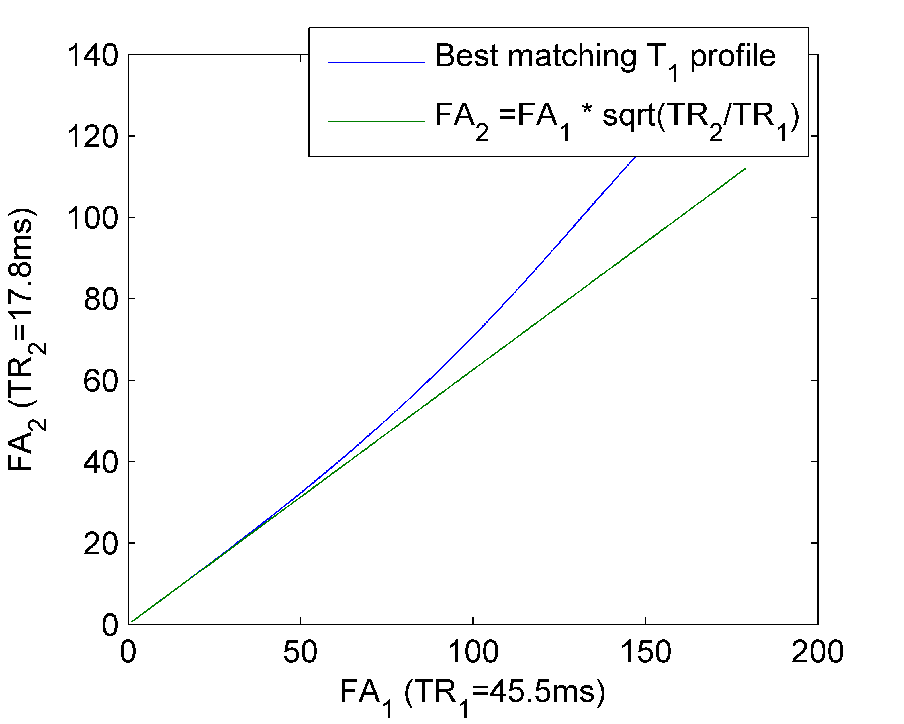
We want to use images with different echo time ( $TE$ ), flip angle( $FA$ ) and repetition time ( $TR$ ) to characterize $f(TE)$ , without having to quantify $T_1$ . Hence we want a relation between $TR_1$ , $FA_1$ , $TR_2$ , and $FA_2$ of two acquisitions such that the ratio of signals is independent of $T_1$ . Unfortunately, no closed form analytic relation obtaining that can be derived. Hence, a local relation with $T_1$ is solved for small $FA$ . A series expansion of that solution in $FA_1$ , $TR_2$ , and $TR_2$ , assuming small $FA$ and $TR<<T_1$ , is given by $FA_2=FA_1 \sqrt{ \frac{TR_2}{TR_1 }} \quad \quad \text{(Eq.2) }$ with an intensity scaling $C = \frac{TR_1 \tan(FA_2/2)}{TR_2 \tan(FA_1/2)} \approx \frac{S(TR_2, FA_2)}{S(TR_1,FA_1)} \quad \quad \text{(Eq.3)}$ between the images. Note that Eq.[2] is independent of $T_1$ and hence images satisfying this relation satisfy it for tissues with any $T_1$ .

Experiments

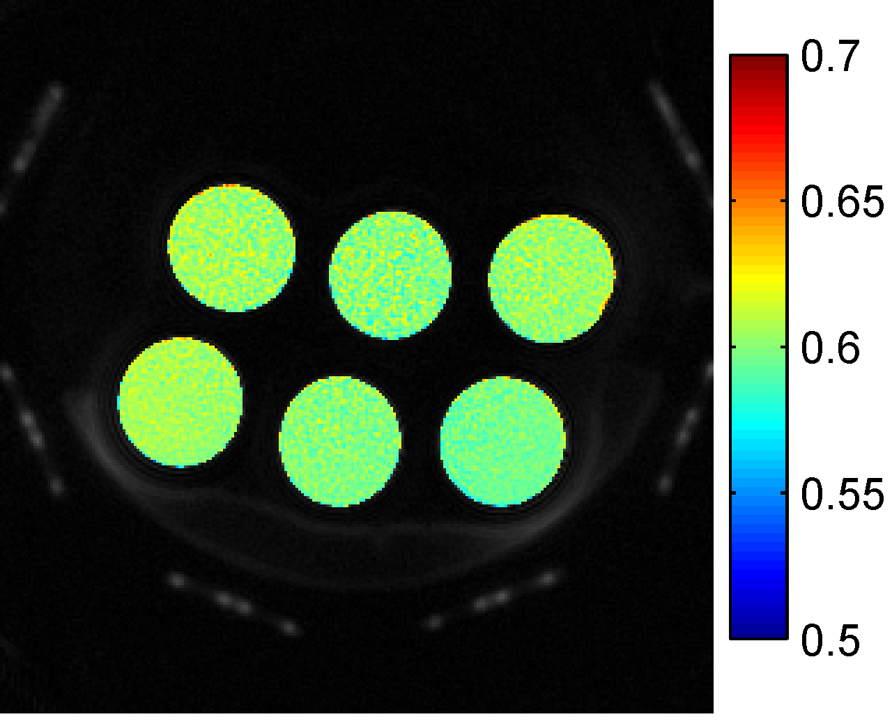
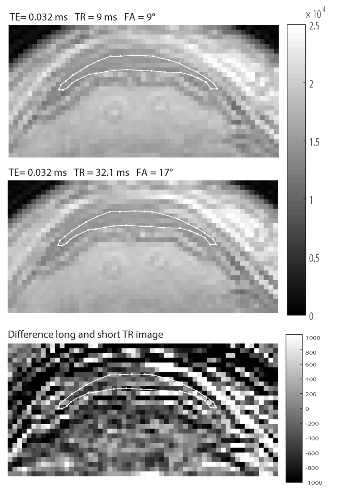
The applicability of Eq.[2] is investigated by comparing with a simulation experiment evaluating S for

$T_1=100-2000ms$ , numerically finding the best matching

$FA_2$ . Experimental validation is obtained with a 3T MRI scanner (GE, Discovery MR750, GE Healthcare), by acquiring two images (

$TR_1/FA_1=45.5ms /8°$ ,

$TR_2/FA_2=17.8ms /5°$ , with

$TE=0.032ms$ ,

$C=0.6246$ , voxelsize=0.586×0.586×2.00 mm3, FOV=150×150×64mm3) of a phantom consisting of 6 tubes differing in

$T_1$ (238-1312ms) and

$T_2$ (17-49ms)[2]. In vivo validation was obtained with two UTE scans of a patellar tendon with

$TR_1/FA_1= 9 ms/9°$ ,

$TR_2/FA_2= 32.1 ms/17°$ ,

$TE=0.032 ms$ .

Results and discussion

Figure 1 shows equation 3 and the numerical solution. Up to $FA_1=39°$ , the approximation holds to good accuracy; $<0.5°$ difference in FA. Using the numerical optimized values, the errors as quantified with $\frac{S(TR_1,FA_1 ) C-S(TR_2,FA_2)}{S(TR_1,FA_1 ) C+S(TR_2,FA_2) }$ are less than 0.06% for all FA and $T_1$ .

Figure 2 shows the ratio of the phantom images. It shows that this ratio is independent of the $T_1$ and approximately 4% below the expected C. This small mismatch could be due to imperfect spoiling as the phantom does not have short $T_2^*$ . However, the difference is constant throughout the image and hence it can be compensated by an additional calibration.

Figure 3 shows an in-vivo validation of the relation. The scaled axial views of a single UTE image of the two acquisitions differing in FA and TR are essentially equal; the difference image shows mainly zero mean noise inside the tendon, which is indicated by a contour. Note the factor 12.5 difference in intensity scale. Some residual motion might cause the main edge artifacts seen in the difference image.

Conclusions

In this work we derived a relation between FA and TR that will allow combining UTE scans with different TR, without requiring knowledge on

$T_1$ or

$T_2$ . This will enable, in the same scan time, increasing the number of short TE scans to better characterize the decay of short

$T_2^*$ species.

Acknowledgements

No acknowledgement found.

References

M.A. Dieringer, M. Deimling, D. Santoro, J. Wuerfel, V.I. Madai, J. Sobesky, F. von Knobelsdorff-Brenkenhoff, J. Schulz-Menger, T. Niendorf Rapid Parametric Mapping of the Longitudinal Relaxation Time T1 Using Two-Dimensional Variable Flip Angle Magnetic Resonance Imaging at 1.5 Tesla, 3 Tesla, and 7 Tesla, PLOS ONE, 2014, 9(3), e91318-e91318
P. Baron, D.H.J. Poot, P.A. Wielopolski, E.H.G. Oei, J.A. Hernandez Tamames Accuracy of ADC measurements with an Ultrashort Echo Time Diffusion Weighted stimulated echo 3D Cones sequence, ISMRM 2017, program nr. 3452

Figures

Figure 1: Derived analytic relation and numerical simulation results.

Figure 2: Ratio of FA2 image/ FA1 image. For all tubes this should be C=0.6246 for TE=0.032ms.

Figure 3: In-vivo 1/C scaled axial images of the patellar tendon and the difference between the short and long TR acquisitions.

Proc. Intl. Soc. Mag. Reson. Med. 26 (2018)

2661