2562
A comparison of biexponetial fitting and spectral modelling methods for T2 mapping of prostate cancer1CRUK Imaging Centre, Institute of Cancer Research, London, United Kingdom, 2MRI Unit, The Royal Marsden NHS Foundation Trust, Sutton, United Kingdom
Synopsis
Spectral modelling and model fitting were compared for quantitative T2 mapping of the prostate. 32-echo data were acquired from 11 patients with biopsy-proven prostate cancer at 3T. There was excellent correlation between the two approaches for estimates of T2-short, T2-long and luminal water fraction (r=0.96, 0.71, 0.94 respectively). Luminal water fractions were significantly higher in normal peripheral and transition zones using the model fitting approach (P = 0.04 and <0.01 respectively), but were comparable in tumor. The larger quantitative difference between tumour and normal tissue could mean model fitting is superior for qualitative assessment in prostate cancer.
Background
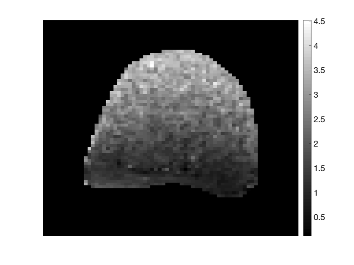
The percentage of luminal space differs significantly between normal and malignant prostate tissue. This difference can be illustrated with quantitative T2 mapping of the prostate, where mono-exponential decay characterises prostate cancer and biexponential decay characterises normal tissue1,2. Quantitative estimation of T2 relaxation is performed by analysing data collected over a range of echo times. However, to capture the longer relaxation times observed in this setting long echo times are required, which implies that the noise floor may be reached in some voxels . The level of noise affects the T2 estimation accuracy, and it is known that noise levels vary spatially when endorectal coils are used (Fig 1). Models that do not explicitly account for the noise floor and its spatial variation could therefore be subject to estimation errors. Multi-exponential model fitting to the data with an appropriate noise model would allow the noise floor to be accounted for, and could therefore be preferable to spectral modelling methods3. The purpose of this study was therefore to compare model fitting and spectral modelling approaches for quantitative T2 mapping of the prostate.Methods
Data Acquisition: 11 patients with biopsy-proven prostate cancer who had 3T endorectal MRI that included T2-weighted images and T2 multi-echo data GRASE acquisitions were studied with IRB approval. Sequence parameters for the multi-echo data were as follows: repetition time msec/echo time msec, 3000/25; number of echoes, 32; field of view, 200 x 200; voxel size, 1 x 1 x 2.5 mm3; imaging matrix size, 160 x 156; reconstruction matrix size, 224 x 224; slice thickness, 2.2-2.5 mm; flip angle, 90°; number of averages, one and imaging duration, 784 seconds.
Data Analysis Tumor region of interests (ROI) were drawn on T2W images by an experienced radiologist around low signal-intensity lesions on T2-W imaging that showed diffusion restriction in biopsy positive sectors of prostate. Multi-echo T2 data were analysed using the spectral modelling approach described previously by Sabouri et al.3 to give estimates of T2‑long, T2‑short, luminal water fraction (LWF) and number of exponential components. In addition the multi-echo data in each voxel were fitted with mono- and bi-exponential decays assuming a Rician noise model, and the scale parameter of the Rician noise (related to the noise standard deviation) was also estimated per voxel. The Bayesian information criterion (BIC) was used to determine the number of exponential components by discriminating between mono- and bi-exponential decays for each voxel, and the BIC calculation accounted for the Rician noise distribution. Correlation between the two analysis methods was performed using Pearson’s correlation coefficient. Parameter values for T2-short, T2-long, luminal water fraction and number of components, N, were compared between the two analysis methods using a paired t-test, with P < 0.05 considered statistically significant.
Results and Discussion
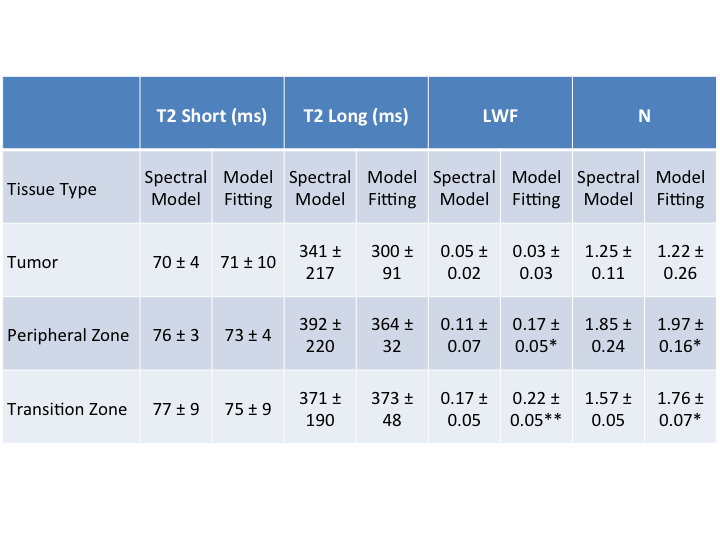
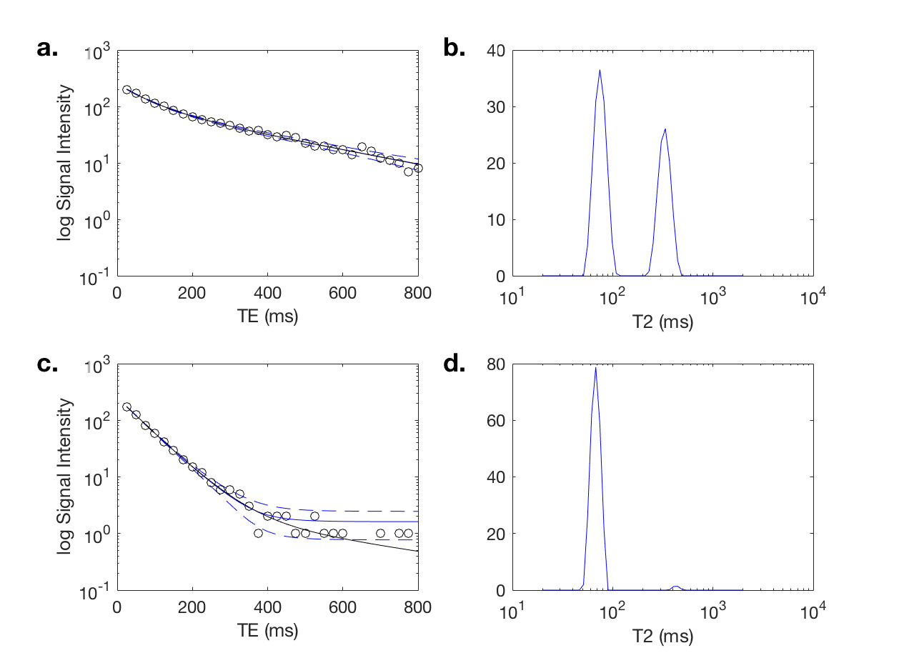
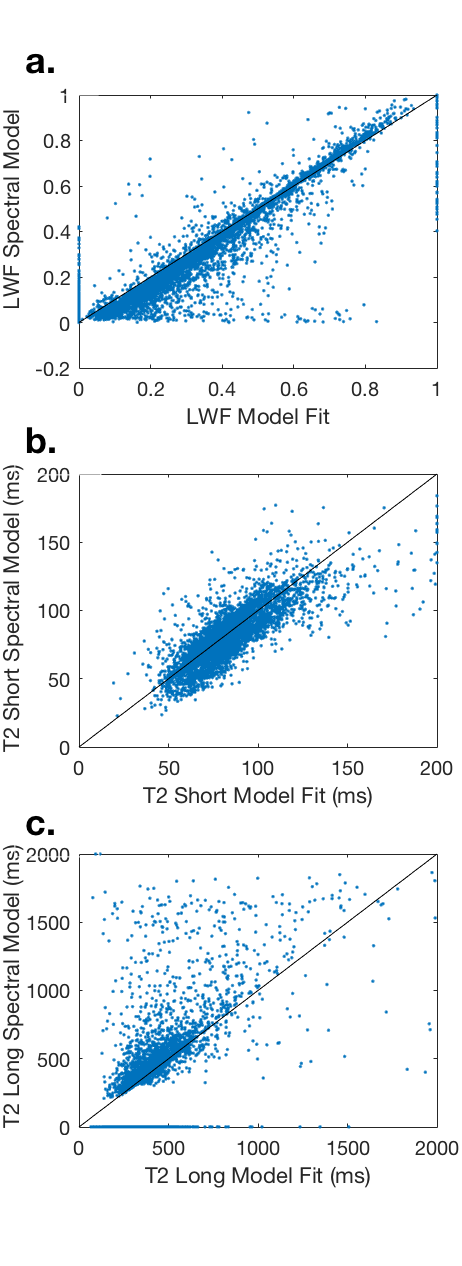
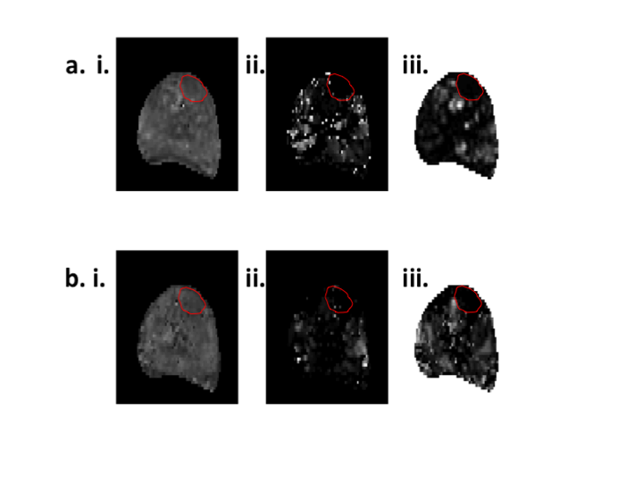
Representative examples of the two analysis methods are shown in Fig. 2. The attenuation curve for the spectral model fit corresponds well with the model fit for voxels where the noise floor is not reached for later echo times (Fig. 2a), however the two curves diverge at later echo times when the noise floor is reached (Fig. 2c). There was excellent correlation between the two approaches for T2-short (r = 0.96), T2-long (r = 0.71) and the luminal water fraction (r = 0.94) across the whole prostate (Fig. 3). Quantitative values for T2 short, T2 long, luminal water fraction and N are given for each analysis approach in Table 1 for tumor, peripheral zone and transition zone. Luminal water fractions were significantly higher for the model fitting approach in the transition zone (P < 0.01) and peripheral zone (P = 0.04), but were comparable in tumor. Similarly, the number of components estimated by data fitting were significantly higher using the data fitting approach but were comparable in tumor. The larger luminal water fractions in the model fitting approach for normal tissue led to increased contrast between tumor and normal tissue (a representative example is shown in Fig. 4).Conclusion
The increased contrast between malignant and non-malignant tissue for luminal water fraction maps may make model fitting that includes a spatially varying noise estimate more suitable for qualitative and quantitative analysis than spectral estimation methods.Acknowledgements
CRUK and EPSRC support to the Cancer Imaging Centre at ICR and RMH in association with MRC and Department of Health C1060/A10334, C1060/A16464 and NHS funding to the NIHR Biomedical Research Centre and the Clinical Research Facility in Imaging.References
1. Storås TH, Gjesdal KI, Gadmar ØB, Geitung JT, Kløw NE. Prostate magnetic resonance imaging: multiexponential T2 decay in prostate tissue. J Magn Reson Imaging. 2008 Nov;28(5):1166-72.
2. Kjaer L, Thomsen C, Iversen P, Henriksen O. In vivo estimation of relaxation processes in benign hyperplasia and carcinoma of the prostate gland by magnetic resonance imaging. Magn Reson Imaging. 1987;5(1):23-30.
3. Sabouri S, Chang SD, Savdie R, Zhang J, Jones EC, Goldenberg SL, Black PC, Kozlowski P. Luminal Water Imaging: A New MR Imaging T2 Mapping Technique for Prostate Cancer Diagnosis. Radiology. 2017 Aug;284(2):451-459.
Figures