Synopsis

An automated method is proposed for generating an optimal preconditioner for a given field input for performing preconditioned total field inversion quantitative susceptibility mapping. In gradient echo data acquired in healthy subjects and patients in various anatomic regions, the obtained preconditioner leads to the same optimal susceptibility map quality as a manually selected preconditioner.

Introduction

Methods

Algorithm: Preconditioned TFI [1] solves:

$$\chi^*=Py^*\ \ \ \ \ \ s.t. \ \ \ \ y^*= \arg\min_{y}{\Phi(y)}=\arg\min_{y}{\frac{1}{2}\parallel w(f-d*Py) \parallel_{2}^2+\parallel \Lambda M_G\triangledown Py\ \parallel_{1}}\ \ \ \ \ (1)$$

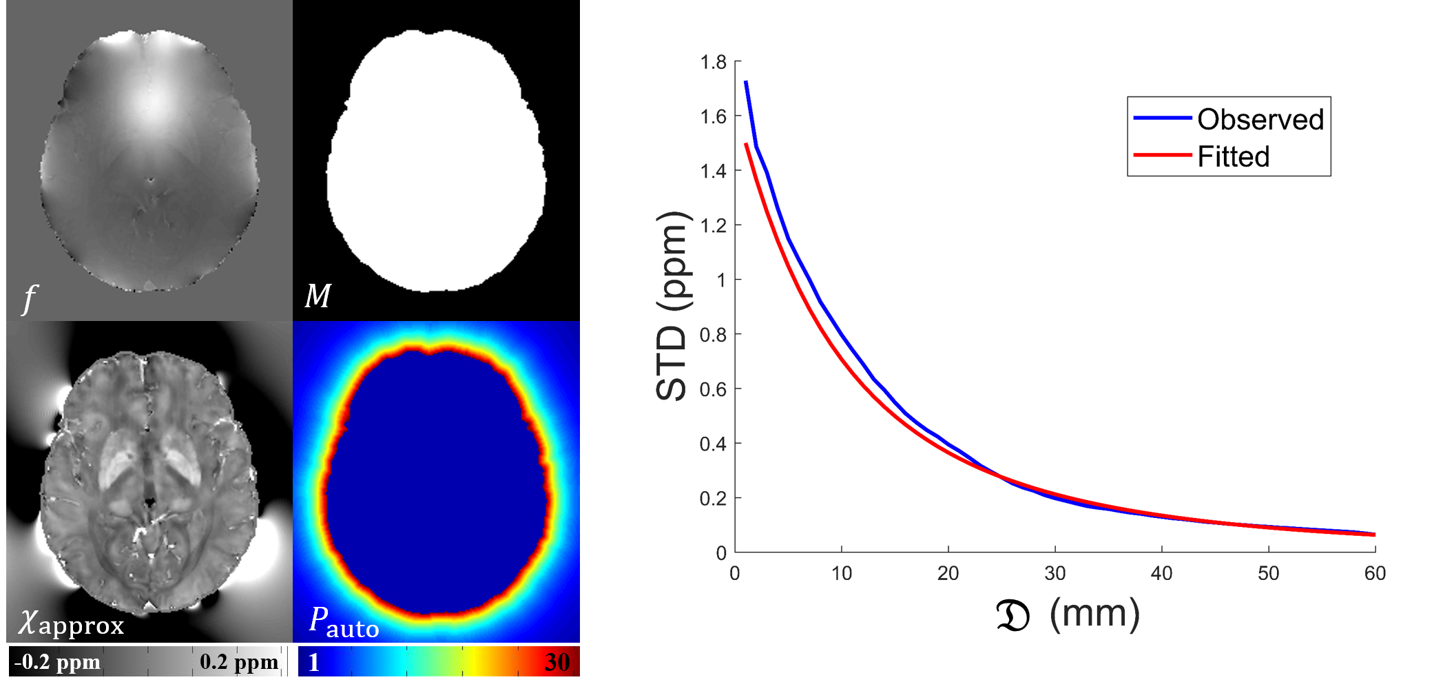
with $$$\chi$$$ the total susceptibility, $$$*$$$ convolution, $$$d$$$ the dipole kernel, $$$f$$$ the total field, $$$w$$$ the noise weighting, $$$\triangledown$$$ the gradient and $$$M_G$$$ the edge weight, $$$\Lambda=\lambda_{1}M+\lambda_{2}\bar{M}$$$ allowing different regularization between soft tissue ($$$M$$$) and strong susceptibility ($$$\bar{M}$$$). This method relies on the fact that convergence is accelerated when the preconditioner approximates the covariance of the solution allowing for whitening [8,9]. Similar ideas were found in [10], where a k-space low-pass filter served as a preconditioner reflecting the spatial smoothness of coil sensitivities. In [1,2], the preconditioner was a binary diagonal approximation to the susceptibility covariance, obtained manually for each type of application. In this work, an approximate solution $$$\chi_{approx}$$$ was used to construct a continuous preconditioner. $$$\chi_{approx}$$$ was obtained by combining the solutions of PDF [3] (using 5 iterations) for $$$\bar{M}$$$ with that of SSQSM [4] for $$$M$$$. $$$\chi_{\bar{M}}$$$ was observed to decay cubically away from the soft tissue boundary. Therefore, $$$\chi_{approx}(\bf r)$$$ was modeled as a Gaussian random field $$$N(0,\sigma ^2(\bf r))$$$, with a spatially varying standard deviation (STD):

$$\sigma (\bf r)=\begin{cases}\ \ \ \ \ \ \ \ \ \ \sigma_1 & {\bf r} \in M\\\sigma_2\left( 1+\frac{D(\bf r)}{r_0} \right)^{-3} & {\bf r} \in \bar{M}\end{cases}\ \ \ \ \ (2)$$

with $$$\sigma_1$$$ and $$$\sigma_2$$$ indicating the STD within $$$M$$$ and $$$\bar{M}$$$, respectively, $$$D(\bf r)$$$ a distance map obtained by calculating the distance between $$${\bf r}\in\bar{M}$$$ and its closest neighbor in $$$M$$$ [5], and $$$r_0$$$ the cubic decay rate. An example is shown in Fig. 1. All parameters $$$(\sigma_1, \sigma_2, r_0)$$$ were fitted to $$$\chi_{approx}$$$ by binning $$$D(\bf r)$$$ into 1mm bins, computing the STD within each bin, and performing a least square fit. $$$\sigma_1$$$ was set to the STD of $$$\chi_M$$$. The preconditioner was defined as:

$$P_{auto} (\bf r)=\begin{cases}\ \ \ \ \ \ \ \ \ \ 1 & {\bf r} \in M\\\frac{\sigma_2}{\sigma_1}\left( 1+\frac{D(\bf r)}{r_0} \right)^{-3} & {\bf r} \in \bar{M}\end{cases}\ \ \ \ \ (3)$$

Note that this is done for each individual input field, as opposed to the previous manual method [1,2].

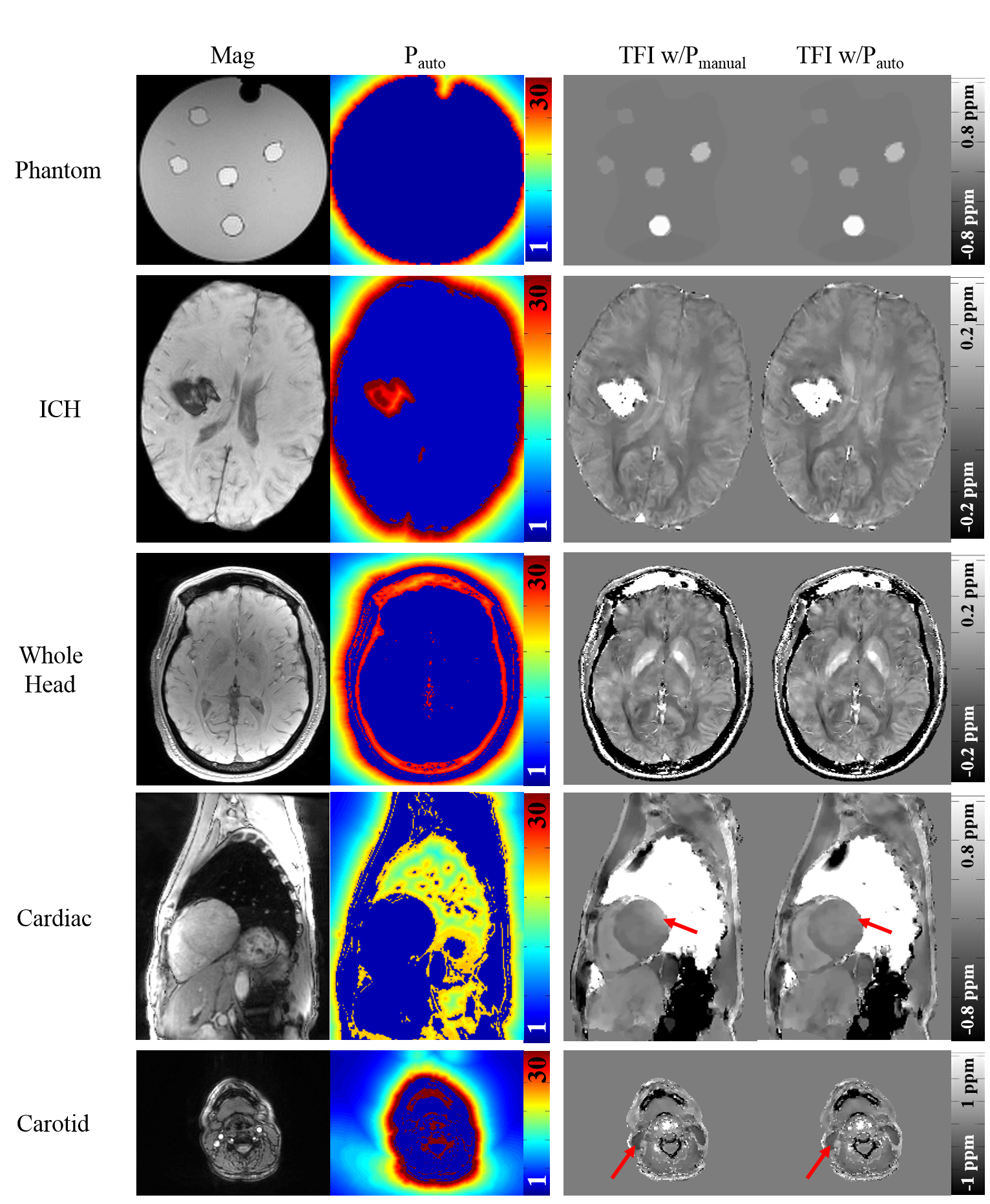
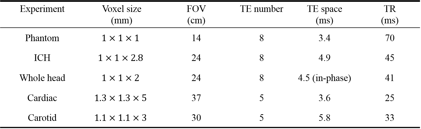
Experiments: 3D gradient echo (GRE) data was acquired on a GE 3T MR750 in A) a phantom with gadolinium-filled balloons (known susceptibilities: 0.05, 0.1, 0.2, 0.4, 0.8 ppm), B) an ICH patient with intracerebral hemorrhage, C) whole head of a healthy subject scanned using in-phase echo spacing, D) heart of a healthy subject scanned using 3D navigator gated GRE sequence, E) carotid of a healthy subject using the same sequence. Detailed scan parameter can be found in Table 1. For data acquired using more than in-phase echoes, SPURS [6] and IDEAL [7] was applied for estimating the total field $$$f$$$ in the presence of fat. The proposed preconditioner was compared with a manually selected preconditioner $$$P_{manual}$$$ [2]: $$$P({\bf r}\in \bar{M})=30$$$ for ICH and head, and 10 for other experiments. $$$\lambda_1=10^{-3}$$$ and $$$\lambda_2=10^{-4}$$$ were used for regularization.

Results

Discussion

Conclusion

Acknowledgements

References

[1]. Liu Z, et al. Preconditioned total field inversion (TFI) method for quantitative susceptibility mapping. MRM. 2017. 78(1):303-315.

[2]. Liu Z, et al. Optimization of Preconditioned Total Field Inversion for Whole head QSM and Cardiac QSM. ISMRM. 2017. p3663.

[3]. Liu T, et al. A novel background field removal method for MRI using projection onto dipole fields (PDF). NMR in BioMed. 2011. 24(9): 1129-1136.

[4]. Bilgic B, et al. Single-step QSM with fast reconstruction. QSM Workshop. 2014. P3321.

[5]. Mishchenko, Y. A fast algorithm for computation of discrete Euclidean distance transform in three or more dimensions on vector processing architectures. Signal, Image and Video Processing. 2015. 9(1):19-27.

[6]. Dong J, et al. Simultaneous Phase Unwrapping and Removal of Chemical Shift (SPURS) Using Graph Cuts: Application in Quantitative Susceptibility Mapping. IEEE Trans Med Imag. 2015. 34(2): 531-540.

[7]. Yu H, et al. Multiecho reconstruction for simultaneous water-fat decomposition and T2* estimation. JMRI. 2007. 26: 1153-1161.

[8]. Calvetti D. Preconditioned iterative methods for linear discrete ill-posed problems from a Bayesian inversion perspective. Journal of computational and applied mathematics 2007. 198(2): 378-395.

[9]. Calvetti D and Somersalo E. Priorconditioners for linear systems. Inverse problems 2005. 21(4): 1397.

[10]. Uecker M, et al. Image reconstruction by regularized nonlinear inversion-joint estimation of coil sensitivities and image content. MRM 2008. 60(3): 674-682.