Introduction

Temporal dynamics of brain’s intrinsic networks have been widely studied using a sliding-window method^{1, 2}. A technical challenge of this method is the proper choice of the window-size. Specifically, a large window may miss existing temporal transients whereas a small window may produce unstable results³. In this study, we describe a new method to determine a time-dependent window-size in a sliding-window analysis. This window-size is calculated from the instantaneous period and energy of each intrinsic mode function (IMF) obtained from empirical mode decomposition (EMD) of each time series^{4, 5}. The IMFs track the local periodic changes of non-stationary time series and can be used to compute an optimum window-size at each time-point. We further incorporate the optimum window-size to explore whole-brain dynamic functional connectivity^2,6 changes in normal controls (NCs) and subjects with Parkinson’s disease (PD).

Methods

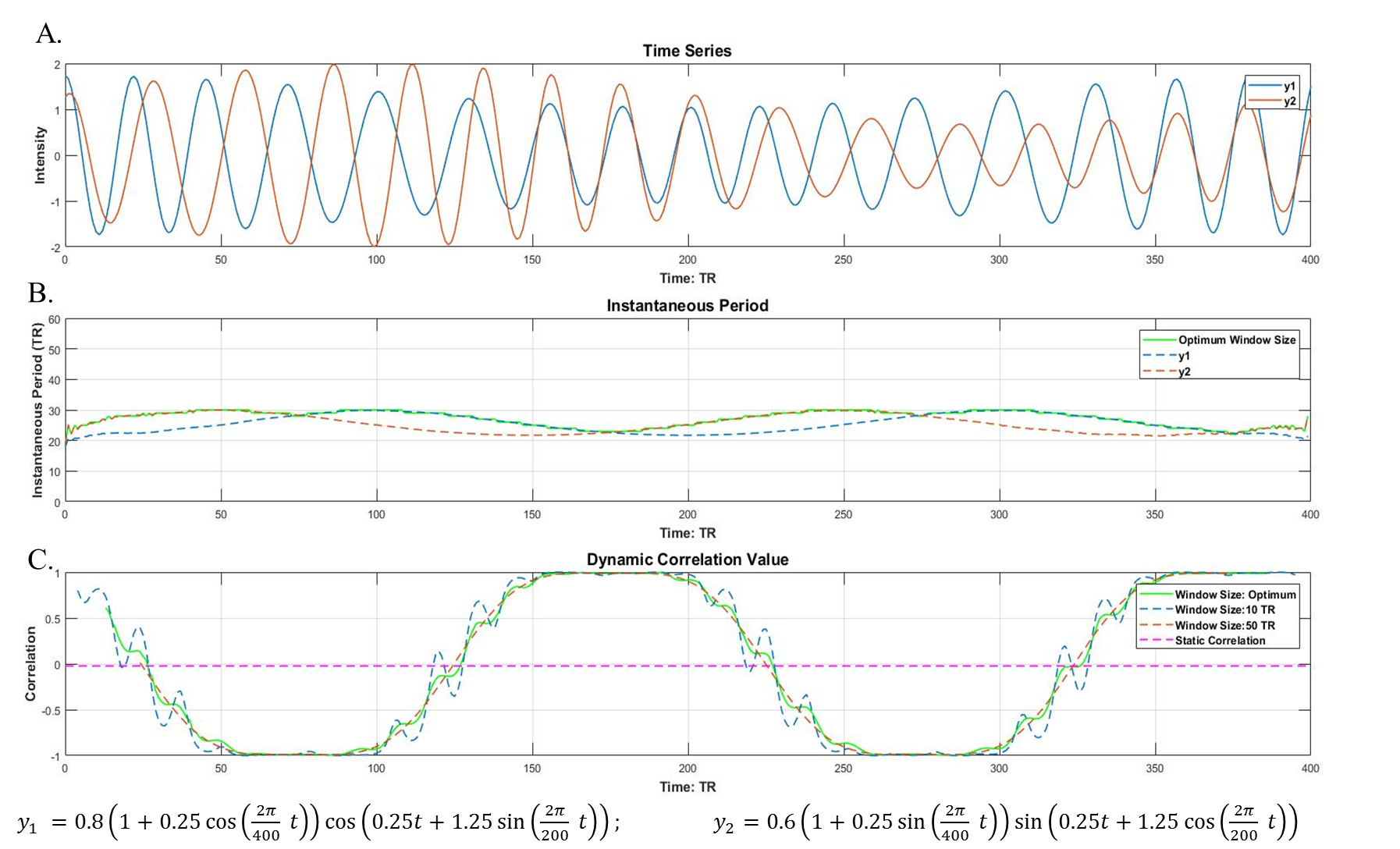
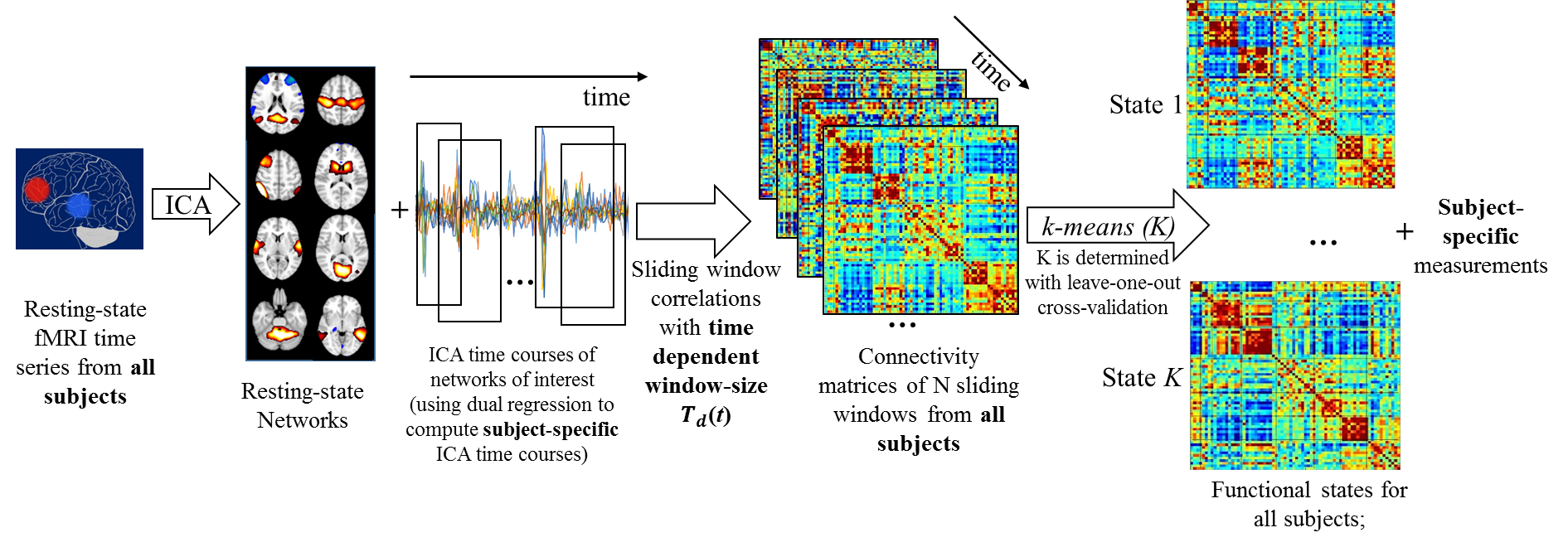
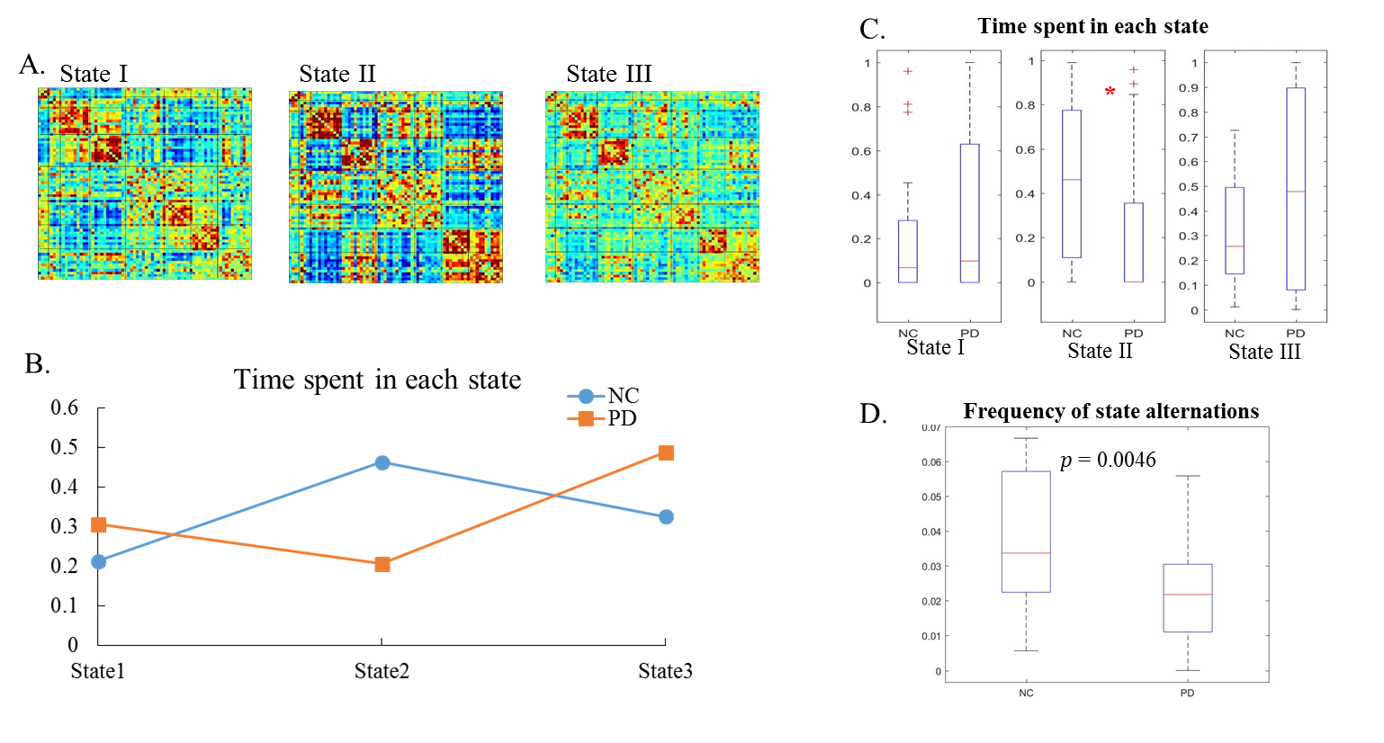
Time-dependent window-size: Given two time series y₁(t) and y₂(t) where t denotes each time point, a time-dependent window-size is determined as follows: Each time course (y_p(t),p=1,2) is first decomposed into different IMFs (c_pi(t)) using EMD^4,5, i.e.y_p(t)=Σ_ic_pi(t)+r_p(t), where r_p(t) are the residuals. The Hilbert transform⁴ is then performed on each IMF to compute the instantaneous period (T_pi(t)) and energy density (E_pi(t)). Next, the time-dependent period (T_p(t)) at every t is determined as an average of T_pi(t) weighted by the energy density E_pi(t) , i.e.T_p(t)=(1/Σ_iE_pi(t))*Σ_i(T_pi(t)*E_pi(t)). The final time-dependent window-size of y₁(t) and y₂(t) to obtain an optimal sliding-window correlation is chosen to be T_d(t)=max(T₁(t),T₂(t)). Simulation: Two non-stationary time series, y₁ and y₂, were simulated at TR = 1s (Fig. 1(A)), with a static correlation of -0.02. The dynamic correlations between y₁ and y₂ were calculated and compared using the sliding-window method with two fixed window-sizes: 10TR and 50TR, as well as the time-dependent window-size T_d(t). Real fMRI data: We studied data from 18 NCs (14 Males; 64.25±9.50 years) and 20 de-novo PD patients (11 Males; 58.03±11.54 years; UPDRS-III: 15.05±7.43) obtained from Parkinson’s Progression Markers Initiative (PPMI) database⁷. Resting-state fMRI were performed on 3T Siemens scanners (TR/TE/Flip Angle/Resolution=2.4s/25ms/80deg/3.3mm³, 210 time-frames) and went through standard preprocessing steps. Whole-brain dynamic functional connectivity analysis with the time-dependent window-size: A flow chart of our analysis is presented in Fig. 2. First, a group ICA with 100 components was carried out using fMRI time-series from both PD and NC subjects. 72 components were identified as network-related components and the corresponding subject-specific ICA maps and time courses were calculated using dual-regression. The whole-brain dynamic connectivity matrices were calculated using sliding-window correlations between pairwise subject-specific ICA time series with the time-dependent window-size T_d(t). The connectivity matrices in each sliding-window were then concatenated in time for each subject, and further stacked for both PD and NC subjects. K-means clustering was performed on the concatenated connectivity matrix from all subjects to estimate dynamic functional states for both groups. The optimum cluster number k was determined by the leave-one-out cross-validation. Finally, the time spent in each state and the frequency of state alternations were calculated for every subject separately and used to compare the temporal dynamics between the PD and NC groups.

Results

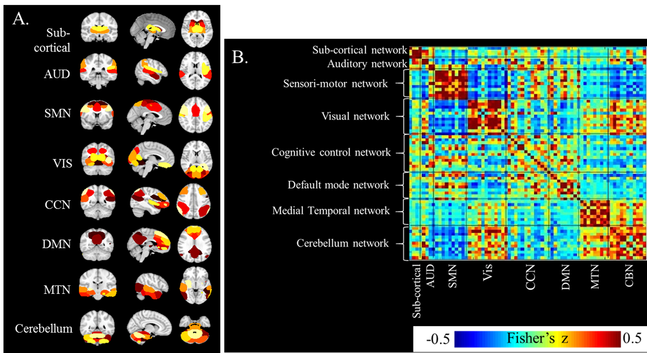
The dynamic correlations between the two simulated time series (Fig.1(A)) were calculated using different window-sizes (Fig.1(B)). Compared to the fixed window-size (dashed lines, Fig.1(C)), the time-dependent window (solid line) captures local transients and avoids unstable fluctuations in calculating correlations. Fig. 2 shows the flow chart of our whole-brain dynamic connectivity analysis with time-dependent window-size. Static correlation within and between each network (Fig.3(A)) are revealed by Fisher’s z statistics and shown in Fig. 3(B). Three dynamic functional states are determined from the leave-one-out cross-validation in k-means clustering for both PD and NC subjects (Fig. 4(A)). Fig. 4(B) shows that NC subjects spend significantly more time in State II, which has stronger connections, both between and within networks, whereas PD patients tend to stay longer in weaker connected functional states I and III. Furthermore, significant reduced frequency of state alternations (p=0.0046) is found in PD group (Fig. 4(D)), which is not observed when repeat the same analysis with a fixed window-size of 13TR (~30secs) or 20TR (~50secs), as used in previous studies^2,3.

Discussion and Conclusion

Our method determined a time-dependent window-size in a sliding-window method based on local information of IMFs from each ICA time series. The running-correlation computed with a time-dependent window-size was able to capture local transients without creating unstable fluctuations (Fig. 1). By incorporating the optimum window-size in whole-brain dynamic functional connectivity analysis (Fig. 2), we found altered whole-brain temporal dynamics in PD subjects (Fig. 4). This finding corroborates with previously reported electrophysiology data in PD⁸.

Acknowledgements

The study is supported by the National Institutes of Health (grant number 1R01EB014284 and P20GM109025). PPMI is sponsored and partially funded by The Michael J. Fox Foundation for Parkinson’s Research (MJFF). Other funding partners include a consortium of industry players, non-profit organizations and private individuals (for a full list see http://www.ppmi-info.org/about-ppmi/who-we-are/study-sponsors/).