2299
Modelling the laminar GRE-BOLD signal: integrating anatomical, physiological and methodological determinants1Max Planck Institute for Human Cognitive and Brain Sciences, Leipzig, Germany
Synopsis
An insight into the layered functional organization of grey matter can be offered by spatially accurate high resolution measurements of the laminar BOLD signal. However, their specificity is limited by anatomical, physiological and methodological features affecting the functional point spread function (fPSF). In order to examine these, an integrated model of the laminar GRE-BOLD signal has been formulated that combines a vascular geometric model of the cortex with a model describing the relationship between underlying physiological parameters and R2* changes. Using the new detailed model we are able to characterize the laminar GRE-BOLD signal dependency on physiological and partial volume effects.
Introduction
Spatially accurate high resolution measurements of the laminar BOLD signal may offer insights into the layered functional organization of grey matter. Besides hardware- and pulse sequence-related aspects, the spatial specificity of the measured signal depends on characteristics affecting the functional point spread function (fPSF): anatomical, in particular the distribution of penetrating intracortical vessels, physiological, such as the underlying metabolic state and neurovascular coupling, and the partial volume from adjacent non-cortical tissue. A first approach to the characterization of the laminar fPSF and GRE-BOLD signal has been recently proposed1, allowing for a description of the dependency on the distribution of intracortical veins (ICVs).Novelty and aim
We propose a new detailed model for studying the laminar GRE-BOLD signal. With this we are able to address yet not fully characterised anatomical, physiological and partial volume sources of variability affecting the spatial specificity of the signal.Methods
A vascular cortical model was defined based on that proposed by Markuerkiaga et al.1, here extended to also include intercortical arteries (ICAs). These are comparable in structure and volume to the ICVs, but have a spatial gradient in O2 saturation as well as different vasodilatory properties2. A model relating underlying physiological parameters and values of R2* was also defined, adapting the approach developed by Griffeth et al.3. This allows us to simulate the effect of a wide range of physiological alterations triggered by neural activation and variations in experimental parameters. The two were combined by modelling the O2 concentration dependence on local metabolism, leading to the definition of the integrated model of the laminar GRE-BOLD signal (see diagram and equations in Fig. 1). The synthetic GRE-BOLD signal was simulated for a 7T experiment in the noiseless condition as a stack of 10 “simulation voxels” (0.75x 0.75x0.25 mm3 – third dimension along the cortical depth), spanning across the primary visual cortex perpendicularly to its surface. When evaluating imaging conditions similar to the real-case, “sampling voxels” of 0.75x 0.75x0.5 mm3 were calculated from the previous. We firstly quantified the contribution of the simulated GRE-BOLD signal from the different components of cortical vasculature and characterised the laminar fPSFs. Using the integrated model it was then possible to evaluate how the signal is modulated by changes in the underlying physiology and neurovascular coupling for a given simulated metabolic activation pattern. Two additional compartments were also included in the analysis: the pial compartment, composed of CSF and pial vessels (as per 4), and white matter, composed of parenchyma and vasculature (as per 5). Effects of partial volume were simulated calculating the signal resulting from an offset between the simulation and the lower resolution sampling voxels. A convolution kernel was also applied to account for imaging geometrically complex patches of cortex (see simulation flowchart in Fig. 2).Results
Fig. 3 reports the effects of taking into account ICAs in the simulation. Vascular distributions with and without ICAs are shown in A and B respectively. The laminar fPSFs and the GRE-BOLD signal from an arbitrary activation pattern are also shown (C and E respectively), compared to a vascular model without ICAs (D and F). Differently to the ICVs, the contribution of the ICAs is found to affect the signal both ipstream and downstream through changes in O2 availability. In Fig. 4 effects of changes in underlying physiology and neurovascular coupling are simulated, highlighting dramatic consequences for the contrast between layers given an arbitrary activation pattern both with (top row) and without ICAs (bottom row). Finally the partial volume due to relative shifting of the sampling voxels up to 200 μm is characterised in Fig. 5. Here the dependency of this source of variability on the spatial distribution of the metabolic activation pattern and the predominance of the signal in the upper layer due to the effect of pial vasculature are characterised.Conclusions & Discussion
An integrated model of the laminar GRE-BOLD signal was defined, providing a comprehensive framework for studying spatial specificity of functional imaging. This enabled a more insightful analysis of the spatial modulation induced by the ICAs, physiological and partial volume effects. Besides signal characterisation, the proposed model can be applied both prospectively, to estimate the effect size or contrast between layers achievable with a given experiment, and retrospectively, using fPSFs to filter the measured GRE-BOLD profiles. Future investigations might address the experimental validation of the model and the inclusion of other major sources of nuisance, such as long distance effects of large pial vessels and noise.Acknowledgements
The research leading to these results has received funding from the European Research Council under the European Union's Seventh Framework Programme (FP7/2007-2013) / ERC grant agreement n° 616905.References
1 - I. Markuerkiaga, M. Barth, and D. G. Norris, “A cortical vascular model for examining the specificity of the laminar BOLD signal,” Neuroimage, vol. 132, pp. 491–498, 2016.
2 - S. Sakadžić, E. T. Mandeville, L. Gagnon, J. J. Musacchia, M. A. Yaseen, M. A. Yucel, J. Lefebvre, F. Lesage, M. Anders, K. Eikermann-haerter, C. Ayata, V. J. Srinivasan, E. H. Lo, A. Devor, and D. A. Boas, “margin of oxygen supply to cerebral tissue,” Nat Commun, vol. 5, no. 5734, 2015.
3 - V. E. M. Griffeth and R. B. Buxton, “A theoretical framework for estimating cerebral oxygen metabolism changes using the calibrated-BOLD method: modeling the effects of blood volume distribution, hematocrit, oxygen extraction fraction, and tissue signal properties on the BOLD signal.,” Neuroimage, vol. 58, no. 1, pp. 198–212, Sep. 2011.
4 - M. Bianciardi, M. Fukunaga, P. van Gelderen, J. A. de Zwart, and J. H. Duyn, “Negative BOLD-fMRI signals in large cerebral veins.,” J. Cereb. Blood Flow Metab., vol. 31, no. 2, pp. 401–12, 2011.
5 - J. R. Gawryluk, E. L. Mazerolle, and R. C. N. D’Arcy, “Does functional MRI detect activation in white matter? A review of emerging evidence, issues, and future directions,” Front. Neurosci., vol. 8, no. 8 JUL, pp. 1–12, 2014.
Figures
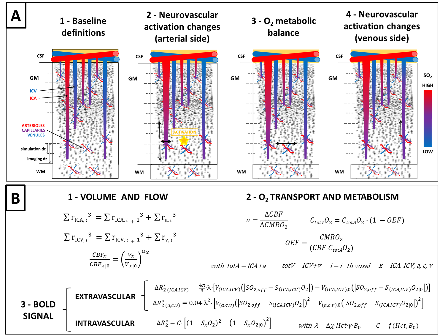
Figure 1 - Vascular model diagram and defining equations.
A: Diagram of vascular model from baseline (1) to activate state (4). SO2 denotes O2 saturation.
B: 1- the radii of ICAs and ICVs (rICA,ICV) are calculated as per 1 and changes in blood flow (CBF) and volume (V) are related by Grubb’s law. 2- O2 metabolism (CMRO2) is related to O2 concentration (C·O2) and O2 extraction fraction (OEF). 3- the BOLD signal is calculated for each vascular compartment as per 3 (please refer therein for notation). Equations valid in any i-th voxel (unless specified), 0 denotes baseline.
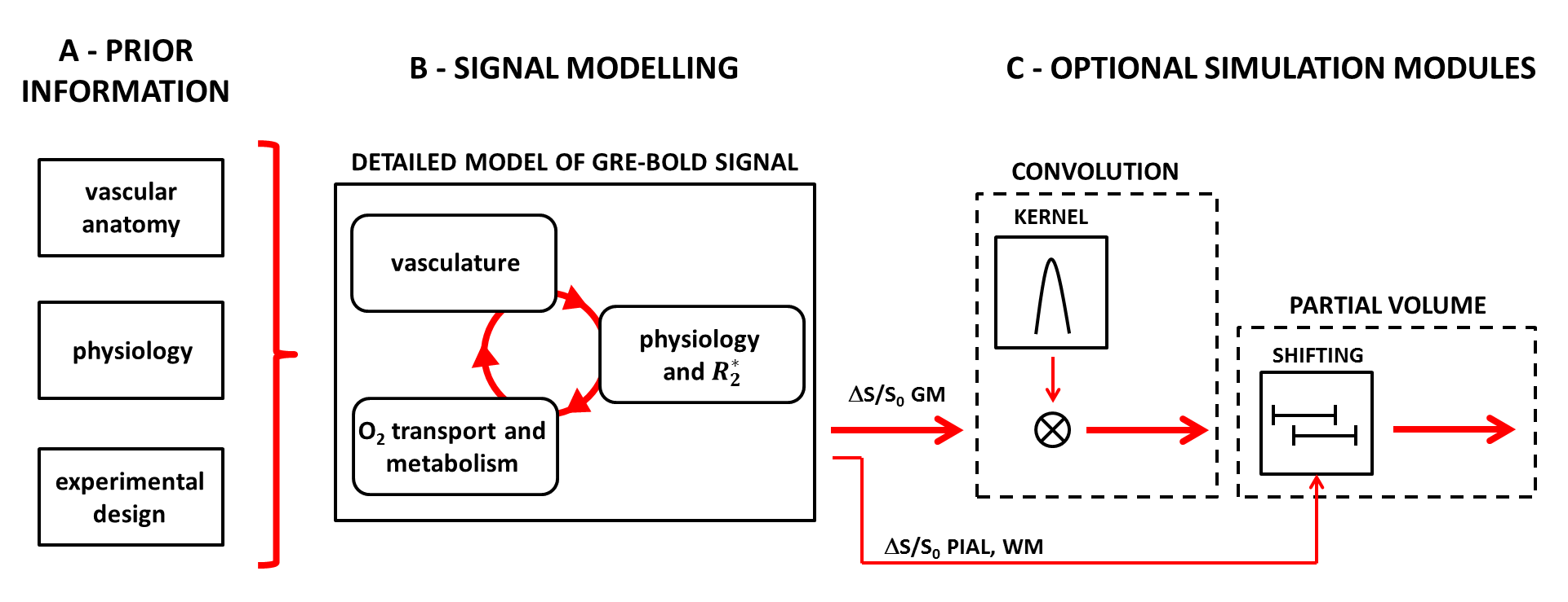
Figure 2 - Simulation flowchart.
A: Details about the vascular anatomy of interest, physiology and experimental design are defined.
B: The simulated GM signal (ΔS/S0 GM) is obtained from the new detailed model of laminar BOLD signal, in which a vascular model (extended from 1) and a model relating physiological changes to ΔR2* (adapted from 3) are coupled by accounting for the O2 transport and metabolism (see Fig. 1).
C: Further optional steps include simulating the effect of imaging a geometrically complex portion of the cortex (CONVOLUTION, as per 1) and PARTIAL VOLUME (both used in Fig. 5).
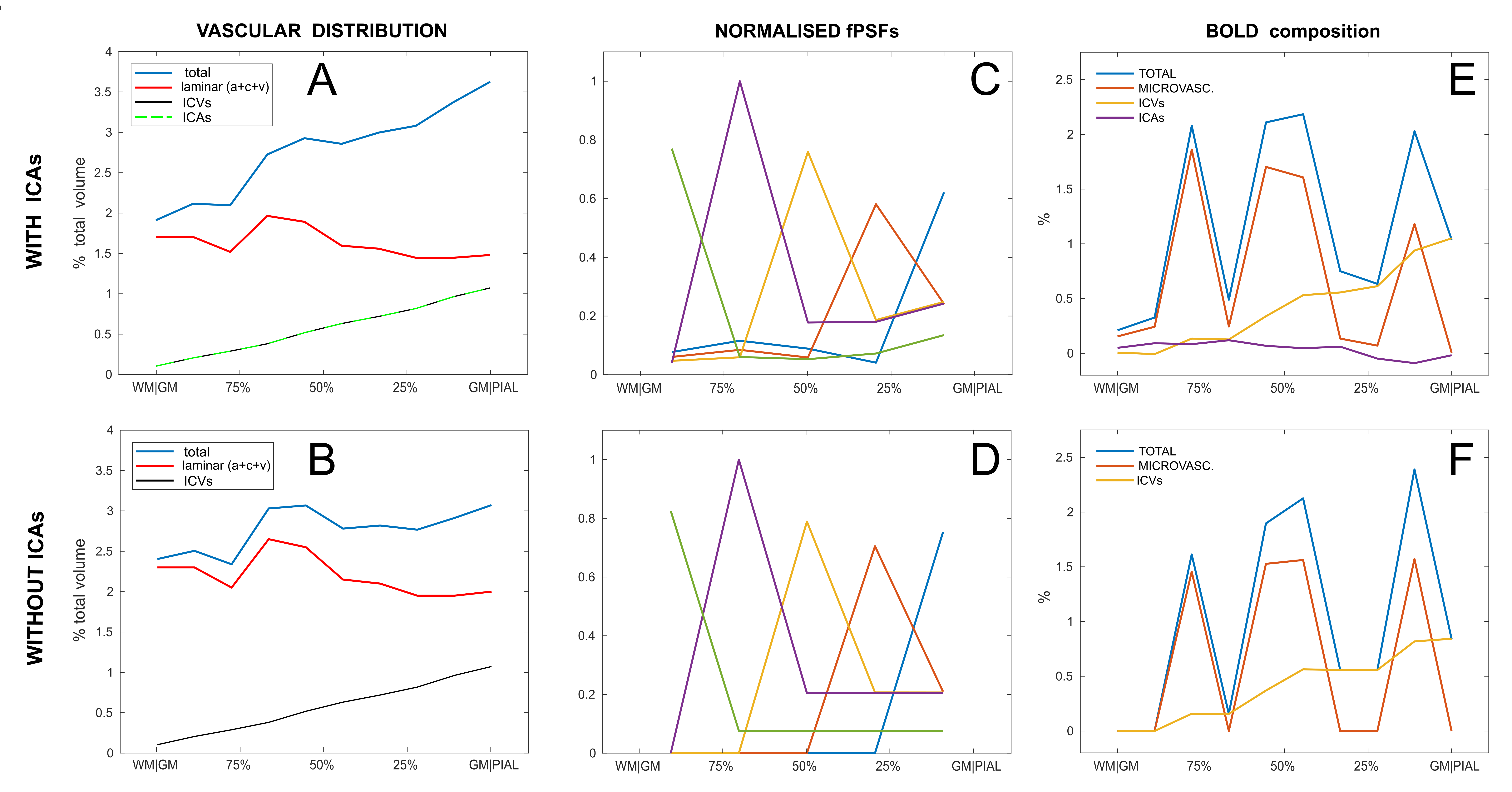
Figure 3 - Accounting for the ICAs in the cortex.
A-B: Vascular distribution across the primary visual cortex with and without ICAs (as per 1). The volume and structure of ICAs was assumed equal to that of the ICVs while the microvascular blood volume (arterioles, capillaries, venules) was decreased to match the total cerebrovascular volume for better comparison.
C-D: calculated fPSFs normalised to the relative maximum value (in the “sampling voxels”).
E-F: BOLD signal composition following for the same arbitrary activation with TE = 28 ms, n (=ΔCBF/ΔCMRO2) = 2, ΔCMRO2 = 20% and OEF0 = 0.4 (for the “sampling voxels”).
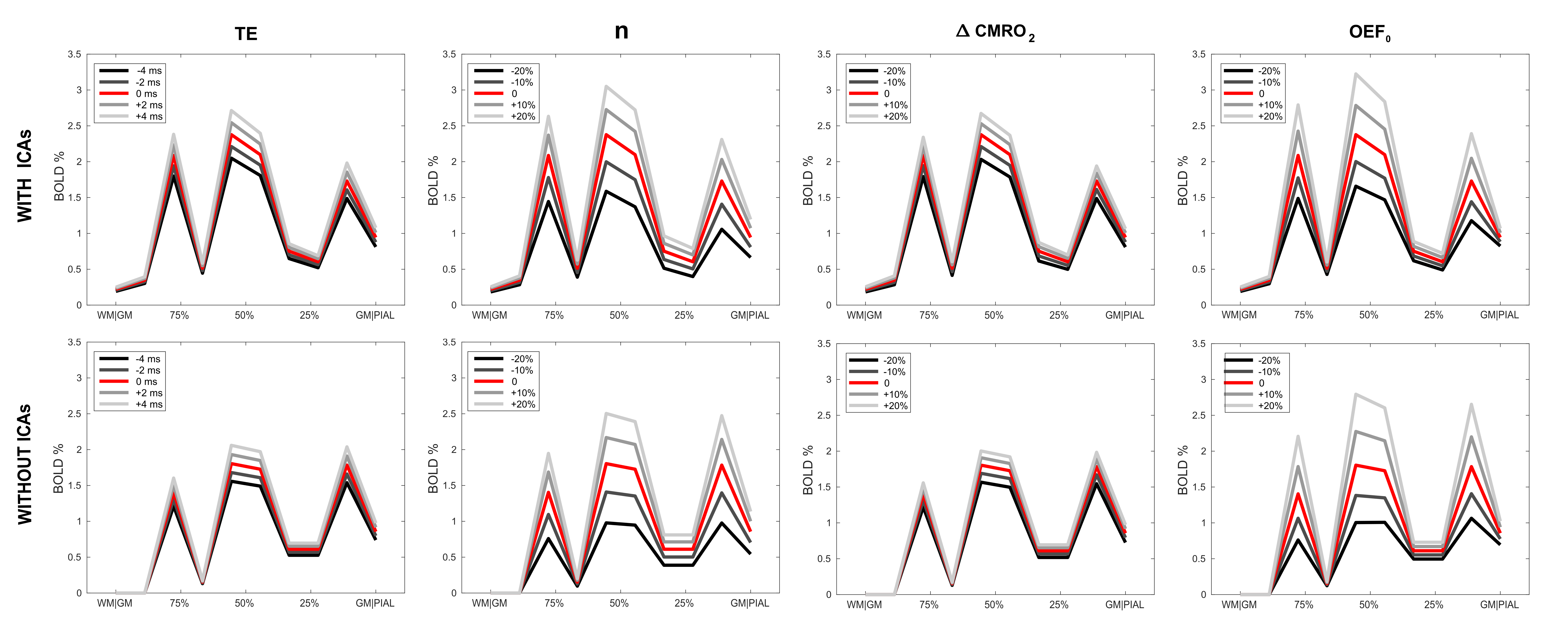
Figure 4 - Effect of variation in experimental and physiological parameters on the BOLD cortical profile.
BOLD signals due to changes in TE, n (=ΔCBF/ΔCMRO2), ΔCMRO2 and OEF0 (baseline oxygen extraction fraction) simulated from the model with and without ICAs (first and second row respectively). Different shades of grey express the change in the relative parameter from the original arbitrary activation (in red – same one as shown in blue in Fig. 2, E-F), with the following values: TE = 28 ms, n = 2, ΔCMRO2 = 20% and OEF0 = 0.4.
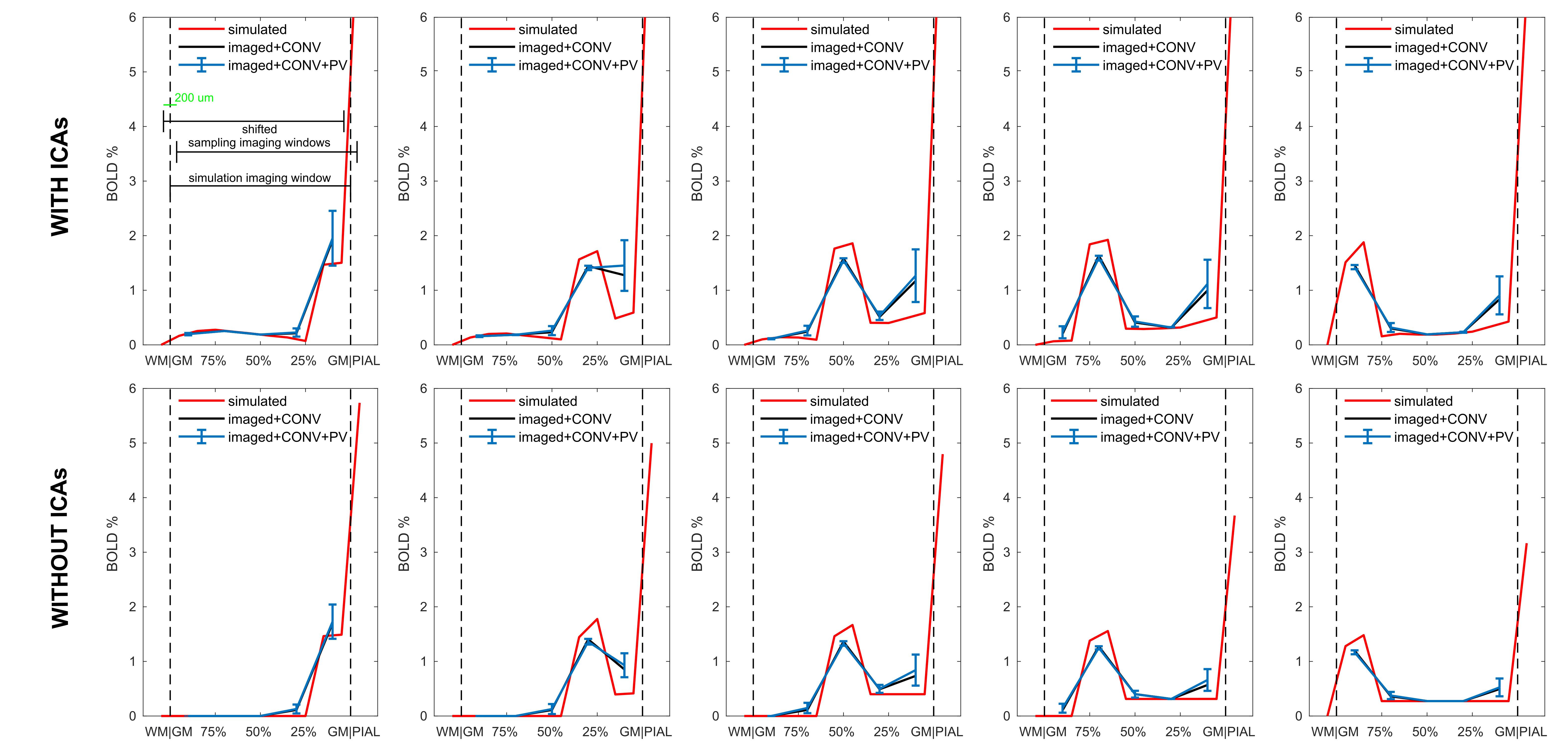
Figure 5 - Approaching the real-case: effects on BOLD laminar profiles.
Simulated BOLD signals following activation from shallower to deeper cortical depth (left to right), with and without ICAs (top and bottom).
Plotted are the signal obtained for GM, WM and PIAL compartments in “simulation voxels” (red), the same signal for “sampling voxels” after convolution (CONV) with a kernel (black) and finally after the effect of partial volume (PV) was simulated (blue, mean and standard deviation bars).
Dashed vertical lines show boundaries between GM, WM and PIAL compartments. Top-left panel: dimensions of the simulation and sampling imaging windows (fully shifted).