2287
Low Frequency Magnetic Resonance Conductivity Imaging By Means of Oscillating Gradient Fields1Department of Electrical and Electronics Engineering, Middle East Technical University, Ankara, Turkey, 2Gaziler Physical Therapy and Rehabilitation Education and Research Hospital, Ankara, Turkey
Synopsis
Recently, low frequency (LF) magnetic resonance electrical conductivity imaging by means of oscillating gradient fields is reported to be infeasible. In these studies, LF phase measurements are modeled with radio frequency (RF) leakage due to geometric shifts in MR images. Although RF leakage is related with conductivity, we have not come across a conductivity image reconstructed using this model. In this study, LF conductivity imaging is evaluated for an MRI pulse sequence including multiple gradient pulses. Geometric shifts are evaluated by focusing on the MR magnitude. A procedure is proposed for the reconstruction of conductivity, based on LF phase measurements.
Introduction
In recent studies, low frequency (LF) electrical conductivity ($$$\sigma$$$) imaging by using oscillating MR gradient fields has been reported as infeasible for conventional spin-echo like MRI pulse sequences1-2. The infeasibility statement is based on radio-frequency (RF) leakage ($$$\Phi_{RF-leak}$$$) model of LF phase ($$$\Phi_{LF}$$$) measurements due to geometric shifts in MR signal1-2. Although $$$\Phi_{RF-leak}$$$ scales with $$$\sigma$$$1-2, we have not observed a $$$\sigma$$$ image reconstructed with $$$\Phi_{RF-leak}$$$. In this study, we evaluate LF conductivity imaging with an MRI pulse sequence including multiple slice selection (SS) gradient pulses. We propose a reconstruction algorithm to recover conductivity images.Methods
Using Maxwell’s equations, fundamental equation of oscillating gradient based LF conductivity imaging can be derived2 as
$$\sigma=\nabla^2{B_{sz}}/(\mu_o\partial{B_{pz}}/\partial{t}), [1]$$
where $$$B_{pz}$$$ and $$$B_{sz}$$$ are the z components of the primary and the secondary magnetic fields created by the gradients and LF induced eddy current ($$${{\bf J}_{LF}}$$$), respectively. Considering a spin-echo pulse sequence with multiple SS gradient (Gz) and 180o RF pulses as shown in Figure 13, $$$B_{sz}$$$ and $$$\Phi_{LF}$$$ are related as
$$\Phi_{LF}=2(N_s-0.5)\gamma{B_{sz}(i,j)}t_r, [2]$$
where $$$N_s$$$ is the number of soft 180o RF pulses, $$$\gamma$$$ is the gyromagnetic ratio of hydrogen, and $$$t_r$$$is the ramp duration. $$$B_{pz}$$$ is determined considering gradient strength ($$$GS$$$), gradient iso-center and slice location. To obtain $$$B_{sz}$$$, $$$\Phi_{LF}$$$ measurements are denoised and scaled. Geometric information is obtained by applying edge detection to MR magnitude image. Quadratic polynomials in horizontal ($$$x$$$) and vertical ($$$y$$$) directions are fitted to $$$B_{sz}$$$ to obtain filtered $$$B_{sz}$$$images. Finally, $$$\sigma$$$ is reconstructed by simplifying Eq. [1] as
$$\sigma=(\frac{\partial^2{B_{sz-x}}}{\partial{x^2}}+\frac{\partial^2{B_{sz-y}}}{\partial{y^2}})/(\mu_o\partial{B_{pz}}/\partial{t}), [3]$$
where $$$B_{sz-x}$$$ and $$$B_{sz-y}$$$are the filtered images. In order to investigate $$$\Phi_{RF-leak}$$$ due to geometric shifts, we focus on MR magnitude images.
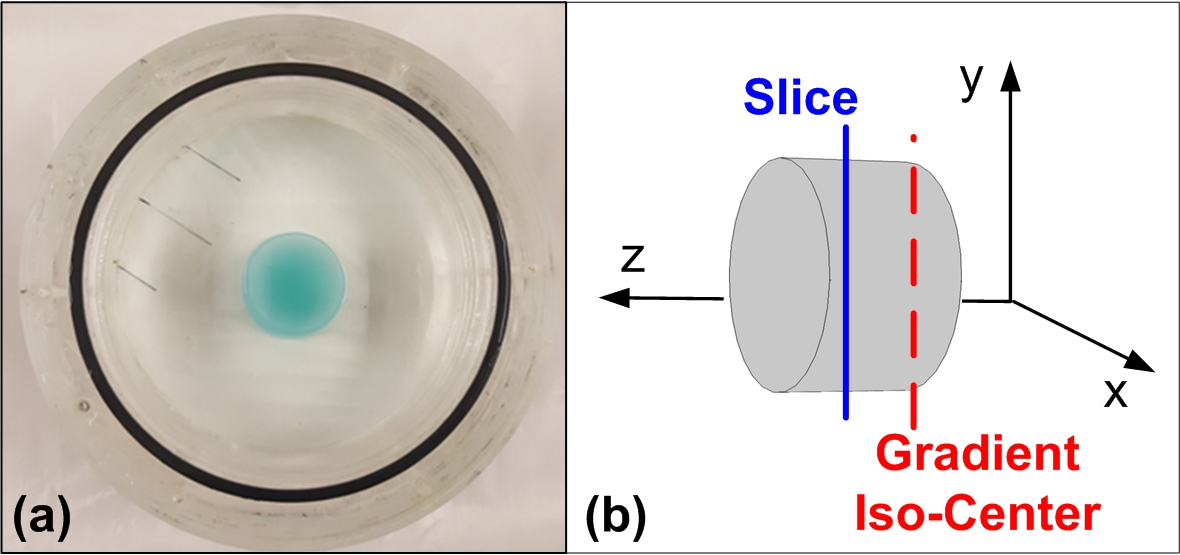
The pulse sequence in Figure 1 is realized on a 3T MRI scanner (Magnetom Trio, Siemens AG, Erlangen, Germany). Transverse (xy) slice with a thickness of 5 mm is selected. Gz is applied with $$$GS=4.8$$$ mT/m and $$$N_s=21$$$. Field of view is 25×25 cm2 with spatial sampling of 128×128 pixels. By applying the pulse sequence twice with positive and negative Gz polarities and taking the difference of resultant $$$\Phi$$$ distributions $$$\Phi_{LF}$$$ is obtained1-3. A cylindrical Plexiglas phantom with a diameter of 19 cm and a height of 10 cm is used as shown in Figure 2. The phantom is filled with a solution of 0.55 g NaCl and 0.05 g CuSO4 in 100 ml distilled water. A cylindrical inhomogeneity with a diameter of 4.8 cm and a height of 10 cm is located inside the phantom. The inhomogeneity is composed of 0.8 g NaCl, 0.05 g CuSO4, 1 g Agar and Tx151 in 100 ml distilled water. Conductivity of the background and the inhomogeneity are 0.75 S/m and 1.2 S/m, respectively.
Results
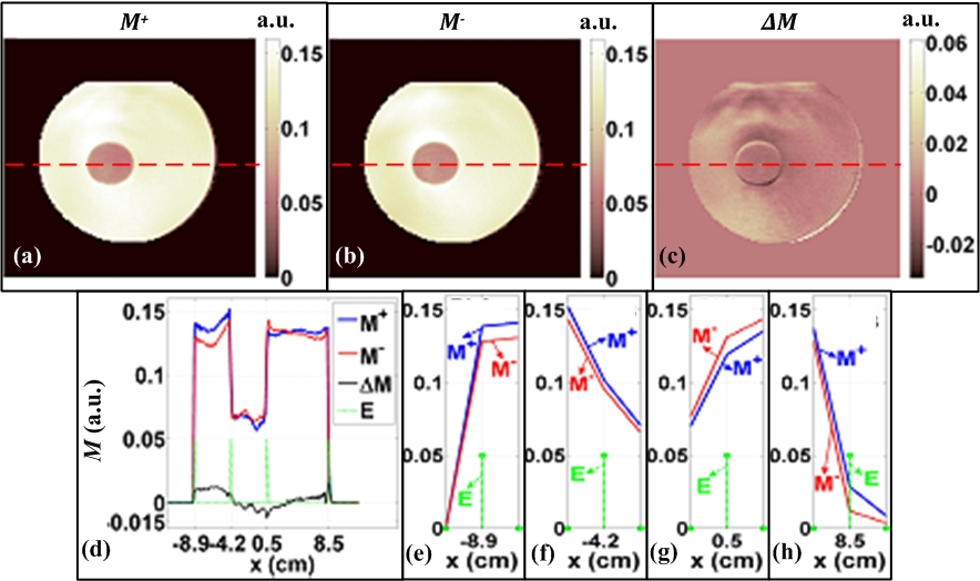
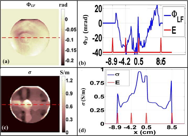
MR magnitude images acquired with positive and negative Gz polarities ($$$M^+$$$, $$$M^-$$$) and their difference ($$$\Delta{M}=M^+-M^-$$$) are shown in Figure 3. $$$M^+$$$ and $$$M^-$$$images exhibit the geometric properties of the phantom. Boundaries of $$$M^+$$$, $$$M^-$$$, and $$$\Delta{M}$$$ are observed at the same locations. $$$\Phi_{LF}$$$ and reconstructed $$$\sigma$$$ images are shown in Figure 4. The range of $$$\Phi_{LF}$$$ profile is close to 60 mrad. Reconstructed $$$\sigma$$$ image and profile exhibit the conductivity properties of the phantom.Discussion and Conclusion
Investigation of $$$M^+$$$, $$$M^-$$$, and $$$\Delta{M}$$$ images reveals the intensity differences. Characteristics of $$$M^+$$$ and $$$M^-$$$ profiles are the same at the boundary pixels. $$$M^+$$$ and $$$M^-$$$ profiles have the maximum and the minimum at the same locations. We can conclude that $$$\Delta{M}$$$ is due to intensity differences rather than geometric shifts. $$$\Phi_{LF}$$$ has quadratic characteristics in the background and the inhomogeneity different from the $$$\Phi_{RF-leak}$$$ model of $$$\Phi_{LF}$$$ distributions in 1-2 which have linear spatial characteristics. Reconstruction of $$$\sigma$$$ images with Eq. [1] and the reported $$$\Phi_{RF-leak}$$$ distributions in 1-2 may not be possible. Reconstructed $$$\sigma$$$ image is a rough approximation of the true $$$\sigma$$$ distribution of the phantom. Boundary artifacts are observed due to $$$\nabla\sigma=0$$$ assumption during derivation of Eq. [1].
We think that switching gradient based LF conductivity imaging should be investigated with MRI pulse sequences including multiple gradient pulses. By this way, $$$\Phi_{LF}$$$ measurements can be increased. Magnetohydrodynamic force created by the interaction of $$${{\bf J}_{LF}}$$$ and static magnetic field ($$$B_o$$$) of the MRI scanner4, diffusion, and drift effects may be sufficiently large to dominate the $$$\Phi_{LF}$$$ measurements, which are close to the phase measurement noise level of MRI scanners5. These flow effects should be investigated in detail in order to master the physics of $$$\Phi_{LF}$$$ measurements even with homogenous Agarose gel phantoms.
Acknowledgements
This study is funded by The Scientific and Technological Research Council of Turkey (TÜBİTAK) and Middle East Technical University (METU) under Research Grants 113E979 and BAP-07-02-2014-007-367, respectively. This work is part of the Ph.D. thesis study of H. H. Eroglu and B. M. Eyuboglu is the thesis supervisor. Experimental data were acquired using the facilities of UMRAM (National Magnetic Resonance Research Center), Bilkent University, Ankara, Turkey.References
1. Mandija S, Van Lier ALHMW, Katscher U, Petrov PI, Neggers SFW, Luijten PR, Van den Berg CAT. A geometrical shift results in erroneous appearance of low frequency tissue eddy current induced phase maps. Magn Reson Med. 2016;76,(3):905-912.
2. Oran ÖF, İder YZ. Feasibility of conductivity imaging using subject eddy currents induced by switching of MRI gradients. Magn Reson Med. 2017;77(5):1926-1937.
3. Eyüboğlu BM, Eroğlu HH, Sadighi MS. An induced current magnetic resonance electrical impedance tomography (ICMREIT) pulse sequence based on monopolar slice selection gradient pulses. Turkish Patent Institute Pending Patent P17/0601.
4. Balasubramanian M, Mulkern RV, Wells WM, Sundaram P, Orbach DB. Magnetic resonance imaging of ionic currents in solution: the effect of magnetohydrodynamic flow. Magn Reson Med. 2015;74(5):1145-1155.
5. Eroğlu HH. Induced current magnetic resonance electrical impedance tomography (ICMREIT) with low frequency switching of gradient fields [PhD thesis]. Ankara, Turkey: Grad Sc. Nat. App. Sci., Middle East Technical University, 2017.
Figures
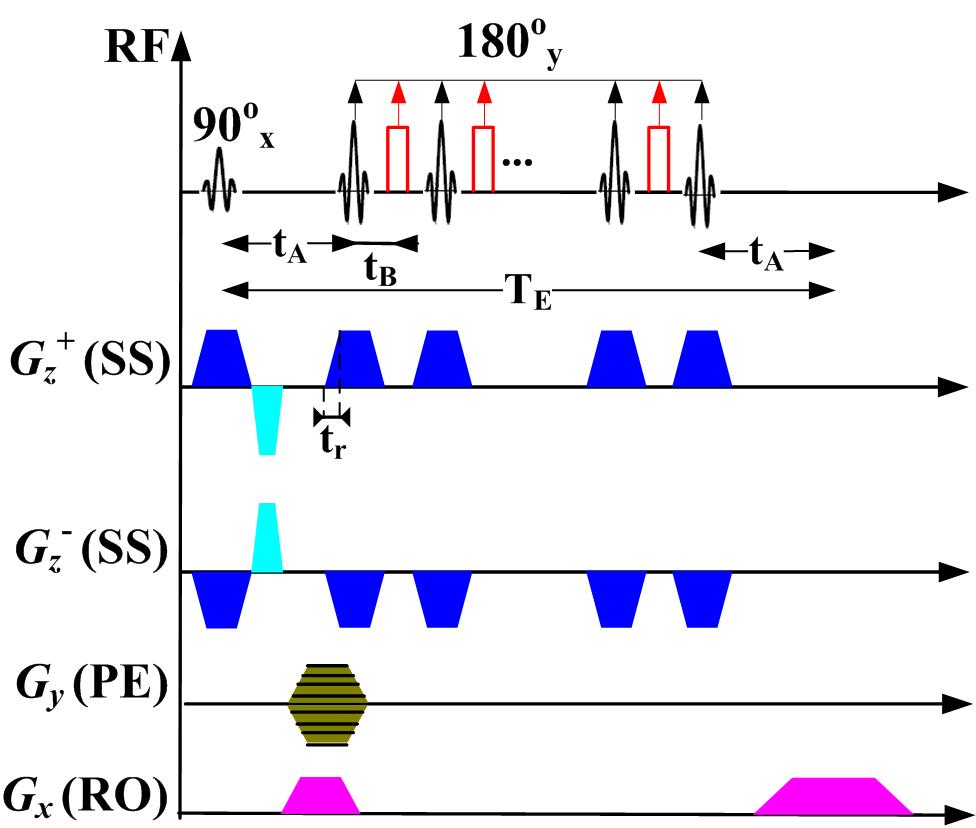
FIG. 1. A spin echo MRI pulse sequence with a switching SS gradient (Gz) waveform. RF is the RF pulse, Gx and Gy are the read-out (RO) and the phase encoding (PE) gradients3.