Synopsis

Magnetic Resonance Elastography (MRE) data show high-amplitude, low frequency artifact which does not accord with the viscoelastic model in near-incompressible tissue. This exploratory study investigates whether the low frequency behavior is poroelastic, and if so whether slow compression wavelengths can be estimated. A cohort of abdominal MRE acquisitions at four frequencies were convolved with a fine-grained Gabor filter bank, and the frequency response of the acquisitions were pooled across subjects for liver and spleen regions. The pooled frequency responses for both liver and spleen showed a shifting peak in the response function mass that tracked with the increase in frequency, with wavespeeds in the shear regime. A second peak identified a lower frequency regime. This regime produced values similar to those observed in tissue poroelastic behaviors.

Introduction

Reconstruction in Magnetic Resonance Elastography usually follows the Navier-Lame equation for isotropic and linearly viscoelastic solids which takes the form $$(\mu(u_{i,j} + u_{j,i}))_{,j} + (\lambda~div~\mathbf{u})_{,i} = \rho \ddot{u}_{i}$$

where $$$\mathbf{u}$$$ is the vector displacement field, $$$\mu$$$ is the shear modulus, and $$$\lambda$$$ Lamé's first parameter. MRE measures the shear wave to determine $$$\mu$$$, while the much longer bulk wave is considered, due to tissue near-incompressibility, too long and fast to measure accurately with typical MRE [1].

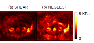
This model predicts that the amplitude of the pressure wave should be $$$\approx \sqrt{10^{3}} \times$$$ less than the shear and arguably neglectable. But as Figure 1 shows, there is a low-frequency artifact of substantial amplitude in MRE data which if neglected will cause large errors in stiffness estimation. Such behavior is better explained by poroelastic theory, which a “slow compression” wave [2]; recent work sets this wave at around 8 m/s in lung tissue [3] which is indeed within the bandwidth of a typical MRE acquisition. The present exploratory study aimed to characterize, analyze and estimate this low-frequency activity in MRE data.

Methods

Subjects - A cohort of 10 abdominal MRE acquisitions were used whose acquisition details can be found in [6]. Driving frequencies of the acquisition were 30, 40, 50 and 60 Hz.

Pre-processing - Data were phase-unwrapped using FSL PRELUDE [4] and then temporally Fourier-transformed. For this initial study only the out-of-plane motion component of the central slice of the abdominal acquisition was analyzed. Masks for liver and spleen were generated using the accompanying T2*-weighted images.

Gabor analysis - A bank of 2D log-gabor filters

$$G(f,\theta) = \exp \left( \frac{-(\log (\omega/\omega_{0}))^2}{2(\log( \sigma_{\omega} /\omega_{0}))^2} \right) \exp \left( \frac{-(\theta-\theta_{0})^2}{2\sigma_{\theta}^2} \right)$$

was developed to enable fine-scale probing of image frequency content. Parameter vectors for the filter bank were: $$$\omega_{0}$$$ = 0.01:0.005:0.2, $$$\theta_{0}$$$ = 0:$$$\pi / 4$$$:2$$$\pi$$$, $$$\sigma_{\omega}$$$ of 0.9 and $$$\sigma_{\theta}$$$ of 0.5. The response at each frequency was calculated by summing voxel-wise the radial components of of each $$$\omega_{0}$$$.

Statistical analysis - Example randomly selected individual voxels within liver and spleen were analyzed. Then, frequency responses were pooled across all subjects by organ using anatomical masks, and peaks in the frequency response curve were determined by using GNU Octave’s findpeaks command in conjunction with a Butterworth high-pass filter (order 4, normalized cutoff 0.05).

Results

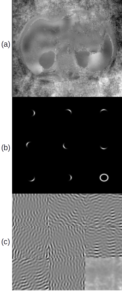
Figure 2 shows the components of the study: (a) is a representative abdominal wave image. (b) shows the filter bank for $$$\omega_{0} = 0.104$$$ normalized frequency: eight directional filters of orientation $$$\theta_{0}$$$ which sum to the ring at bottom right. (c) shows the response of (a) to the filters in (b), leading to the summed response at bottom right.

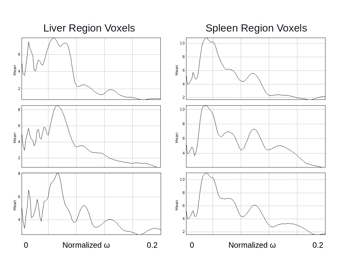
Figure 3 shows the frequency response graph for randomly selected pixels in both liver and spleen regions, for an image at 40Hz: the mass of the frequency response functions is distributed differently by region, but consistently within region: the liver voxels have peak response at $$$\approx \omega_{0} = 0.058$$$ while the spleen voxels have peak response at $$$\approx \omega_{0} = 0.037$$$, which accords with the known higher wavespeeds (therefore lower frequencies) of the spleen.

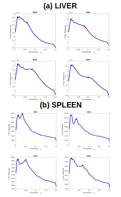
Figure 4 shows pooled frequency response results across all ten subjects by organ, for (a) liver and (b) spleen. Two peaks are again present, and the mass of the second peak increases with frequency, with peaks at 0.035, 0.05, 0.05, and 0.07 for 30, 40, 50 and 60 Hz respectively. The doubling of the peak from 0.035 to 0.07 coincides well with the doubling of the driving frequency from 30 to 60 Hz. These values correspond to wavespeed estimates of between 1.7 m/s and 2 m/s respectively.

The more diffuse higher liver peaks were 0.06, 0.07, 0.08 and 0.1 of normalized frequency respectively(wavespeeds 1 and 1.2 m/s). In all cases the low-regime peak remained between $$$\omega_{0} = 0.01$$$ and $$$\omega_{0} = 0.02$$$, which corresponded to a wavespeed of $$$\approx$$$6.7 m/s.

Discussion

Acknowledgements

References

[1] Manduca, A., Oliphant, T.E., Dresner, M.A., Mahowald, J.L., Kruse, S.A., Amromin, E., Felmlee, J.P., Greenleaf, J.F. and Ehman, R.L., 2001. Magnetic resonance elastography: non-invasive mapping of tissue elasticity. Medical image analysis, 5(4), pp.237-254.

[2] Berryman, J.G., 1980. Confirmation of Biot’s theory. Applied Physics Letters, 37(4), pp.382-384.

[3] Dai, Z., Peng, Y., Mansy, H.A., Sandler, R.H. and Royston, T.J., 2014. Comparison of poroviscoelastic models for sound and vibration in the lungs. Journal of vibration and acoustics, 136(5), p.050905.

[4] Jenkinson, M., 2003. Fast, automated, N‐dimensional phase‐unwrapping algorithm. Magnetic resonance in medicine, 49(1), pp.193-197.