2269
Assessing B1 map errors in vivo: measuring stability and absolute accuracy despite the lack of gold standard1CAMH, Toronto, ON, Canada
Synopsis
B1+ field inhomogeneity is a major source of errors in quantitative mapping. The accuracy of B1 maps, depicting the effects of B1+ inhomogeneity on the flip angle, is thus critical. However, there is no gold standard B1 mapping method in vivo so absolute accuracy is difficult to determine. In this work, we propose steps that exploit known B1 effects in a small phantom to obtain absolute accuracy estimates in vivo. Two B1 mapping methods are required, but neither need be accurate. We demonstrate the proposed assessment by obtaining stability and absolute accuracy measurements of the Method of Slopes B1 maps.
Introduction
At main field (B0) strengths of ≥3T, the transmit radiofrequency (RF) field, B1+, is inhomogeneous, giving rise to local flip angle (α) variations. B1+ inhomogeneity is a major source of error in quantitative parametric mapping methods1-5. The accuracy of B1 maps, which commonly depict the ratio of local to nominal α, is thus critical. Several methods are proposed for B1 mapping, relying on different acquisition sequences and mathematical models of the signal dependence on α and other MR parameters6-10. By acquiring the signal at least twice, with varying parameters, these methods extract α algebraically. The accuracy and stability of B1 maps depend primarily, on how well the model predicts the signal. The robustness of B1 maps can be assessed via simulations11 and mathematical error propagation12, but these approaches do not consider how well the model predicts signal behaviour in vivo. To better assess the stability in vivo, repeat experiments can be performed13. However, due to the lack of a gold standard B1 map in vivo, accuracy is usually measured relatively, i.e., by how much one method varies with respect to another, reference technique. There is no consensus on the reference, thus assessing the accuracy of B1 maps is somewhat arbitrary.
The Method of Slopes (MoS)14 has been proposed as a simple 3D method that yields B1 maps (B1MoS) using an extrapolation to signal null, i.e., exploiting the linearity of the spoiled gradient echo (SPGR) signal vs α relationship as the signal approaches the null point (α=180°). Here, we measure stability and absolute accuracy of B1MoS maps. In doing so, we propose a set of systematic steps that can be used to assess B1 mapping accuracy in an absolute sense, by-passing the lack of gold standard.
Methods
To determine the accuracy of the B1MoS maps, we use a small phantom (relative to the RF wavelength) with flat signal profile and B1=1 expected within. We also rely on any other B1 mapping method. The key is that it does not need to be accurate because we use ratios as follows.
Experiments were performed at 3T (MR750, GE Healthcare) with a receive-only headcoil. The phantom consists of an aqueous MnCl2 solution, with physiological T2 and T1, in small (dia=5cm) and big (dia=9cm) beakers. The phantom and six volunteers were scanned in compliance with the institutional REB. For B1MoS, two full volume 3D SPGR sagittal scans (TR=50ms, (4mm)3 ) were acquired: S3(α=130°) and S4(α=150°)14. A second B1 map was obtained using the stock Bloch-Siegert (BS)10 sequence (B1BS): α =15°, 5mm×(4mm)2 .
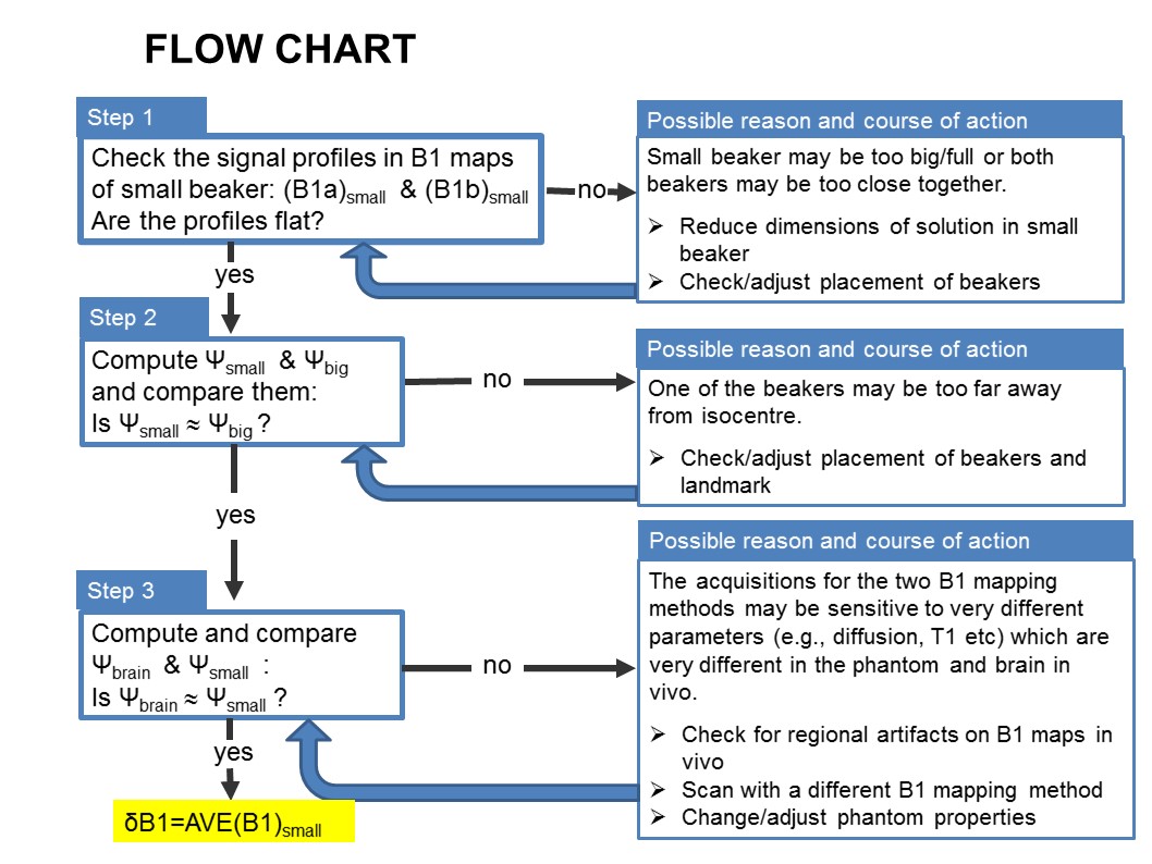
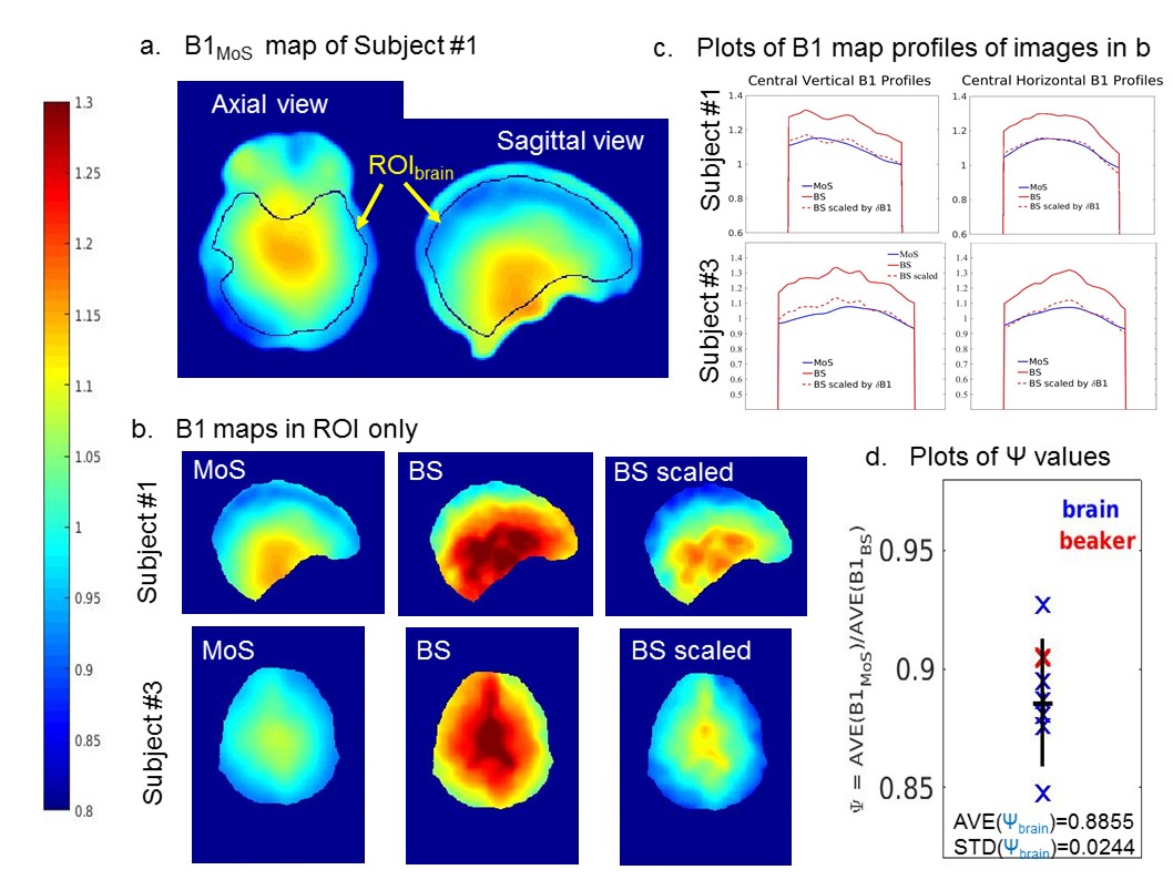
Estimates of absolute B1 error were computed using the small beaker data: δB1=B1measured/B1true=AVE(B1)small/1 for both methods. The ratio was then computed: ψsmall=δB1MoS/δB1BS. Similarly, ψbig=AVE(B1MoS)big/AVE(B1BS)big and ψbrain=AVE(B1MoS)brain/AVE(B1BS)brain were computed for validation (Fig.1). AVE values were taken in regions-of-interest (ROIs) avoiding edges. B1 maps were scaled by ξ=1/δB1 to obtain accurate maps.
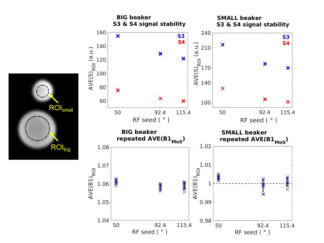
Poor RF spoiling can compromise the SPGR signal. Thus, stability and accuracy of B1MoS was tested on the phantom and two volunteers, at various RF seed (φ) values: 50°, 115.4°, 92.4°. S3 and S4 were acquired three times for each φ, yielding temporal AVE and STD. Nine possible (S3,S4) pairs were used to compute nine B1 maps at each φ. ROIs were used to extract average values in the beakers while voxelwise computations, preserving spatial information, were used in vivo.
Results
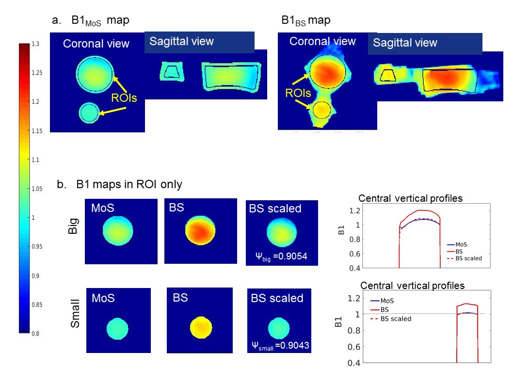
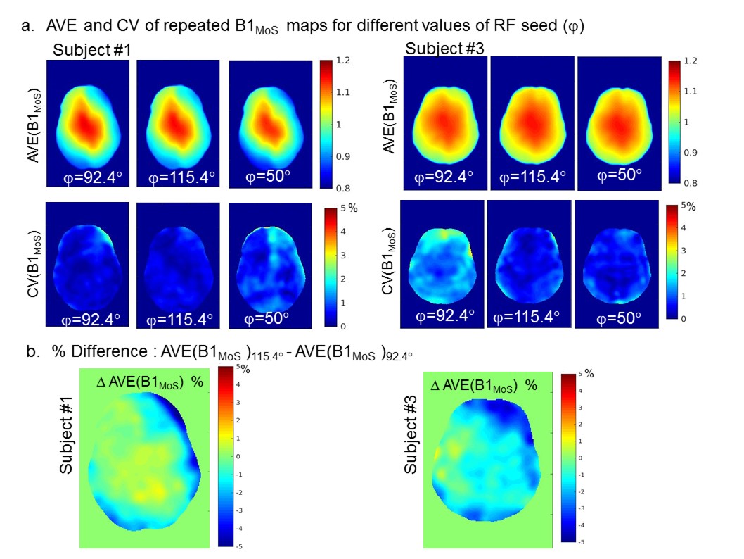
Fig.2 shows plots of the phantom stability results. Fig.3 shows phantom AVE(B1MoS) and AVE(B1BS) maps and profiles, used to assess the accuracy of B1 maps as per flow chart. Fig.4 shows in vivo stability measurements. Fig.5 shows three examples of in vivo B1 map accuracy validation: the results for Ψbrain in all brains are plotted with Ψsmall and Ψbig for comparison.Discussion
Phantom instabilities of S3 and S4 were insignificant. B1 instabilities and inaccuracies were also insignificant and independent of φ: STD(B1)<0.3% ; differences in AVE(B1) across φ were <0.2% despite variations in absolute S3 and S4 (Fig.2). The accuracy of B1maps were: δB1MoS ≈1 (no bias) and δB1BS=1.1058 (≈10% bias) (Fig.3). In vivo, the instability of B1MoS was <2% in most brain regions with highest values for φ=50° (subj#1) and φ=92.4° (subj#3) (Fig.4a). Subj#1 was scanned again and highest instabilities occurred for φ=115.4°, confirming that instabilities are φ-independent and result from motion/physiology. AVE(B1MoS) did not differ significantly with φ in vivo (<2% full brain average) (Fig.4b). ψbrain agreed with phantom values, considering the sensitivity (in particular of B1BS) to physiological effects (Fig.5).Conclusions
We showed systematic steps that yield the absolute accuracy of B1 maps in vivo. B1MoS was found to be both stable and accurate in vivo.Acknowledgements
No acknowledgement found.References
1. Preibisch C, Deichmann R. Influence of RF Spoiling on the Stability and Accuracy of T-1 Mapping Based on Spoiled FLASH With Varying Flip Angles. Magnetic Resonance in Medicine 2009;61(1):125-135.
2. Hurley SA, Yarnykh VL, Johnson KM, Field AS, Alexander AL, Samsonov AA. Simultaneous variable flip angle-actual flip angle imaging method for improved accuracy and precision of three-dimensional T1 and B1 measurements. Magnetic Resonance in Medicine 2012;68(1):54-64.
3. Yarnykh VL. Optimal Radiofrequency and Gradient Spoiling for Improved Accuracy of T-1 and B-1 Measurements Using Fast Steady-State Techniques. Magnetic Resonance in Medicine 2010;63(6):1610-1626.
4. Weiskopf N, Lutti A, Helms G, Novak M, Ashburner J, Hutton C. Unified segmentation based correction of R1 brain maps for RF transmit field inhomogeneities (UNICORT). Neuroimage 2011;54(3):2116-2124. 5. Deoni SCL. High-resolution T1 mapping of the brain at 3T with driven equilibrium single pulse observation of T1 with high-speed incorporation of RF field inhomogeneities (DESPOT1-HIFI). Journal of Magnetic Resonance Imaging 2007;26(4):1106-1111.
6. Yarnykh VL. Actual flip-angle imaging in the pulsed steady state: A method for rapid three-dimensional mapping of the transmitted radiofrequency field. Magnetic Resonance in Medicine 2007;57(1):192-200.
7. Lutti A, Stadler J, Josephs O, et al. Robust and Fast Whole Brain Mapping of the RF Transmit Field B1 at 7T. Plos One 2012;7(3).
8. Stollberger R, Wach P. Imaging of the active B-1 field in vivo. Magnetic Resonance in Medicine 1996;35(2):246-251.
9. Dowell NG, Tofts PS. Fast, accurate, and precise mapping of the RF field in vivo using the 180 degrees signal null. Magnetic Resonance in Medicine 2007;58(3):622-630.
10. Sacolick LI, Wiesinger F, Hancu I, Vogell MW. B-1 Mapping by Bloch-Siegert Shift. Magnetic Resonance in Medicine 2010;63(5):1315-1322
11. Morrell GR. A phase-sensitive method of flip angle mapping. Magnetic Resonance in Medicine 2008;60(4):889-894.
12. Pohmann R, Scheffler K. A theoretical and experimental comparison of different techniques for B1 mapping at very high fields. Nmr in Biomedicine 2013;26(3):265-275.
13. Lutti A, Hutton C, Finsterbusch J, Helms G, Weiskopf N. Optimization and Validation of Methods for Mapping of the Radiofrequency Transmit Field at 3T. Magnetic Resonance in Medicine 2010;64(1):229-238.
14. Chavez S, Stanisz GJ. A novel method for simultaneous 3D B1 and T1 mapping: the method of slopes (MoS). Nmr in Biomedicine 2012;25(9).
Figures