2262
In vivo measurements of T1-dispersion maps in a kidney tumor mouse model using FFC-MRI around 1.5 T1IR4M UMR8081 Univ Paris-Sud CNRS, Université Paris Saclay, Orsay, France, 2IR4M UMR8081 Univ Paris-Sud CNRS, Université Paris Saclay, Villejuif, France, 3Gustave Roussy, Villejuif, France, 4Département d’Urologie – Institut Mutualiste Montsouris, Paris, France, 5Gustave Roussy, Vectorology and Anticancer Therapies, UMR8203 CNRS Univ Paris-Sud, Université Paris-Saclay, Villejuif, France, 6Bio-Medical Physics, School of Medicine, Medical Sciences and Nutrition, University of Aberdeen, Aberdeen, United Kingdom, 7CRMBM UMR7339 CNRS Aix-Marseille Université, Marseille, France
Synopsis
Fast Field Cycling MRI offers the possibility to explore new contrasts generated from NMR dispersion (NMRD) profiles of tissue. Exploiting the dispersion properties of tissues may provide an additional biomarker of diseases through a deeper understanding of molecular mobility. Kidney tumors and healthy kidneys were analyzed among a cohort of twenty-seven mice to give insight into the potential of FFC-MRI for clinical applications. Here, we present R1-dispersion maps performed around 1.5 T to show that the intrinsic dispersion of tumors measured in vivo differs from the one of healthy kidneys.
Introduction
Fast Field Cycling (FFC) enables to measure the evolution of the longitudinal relaxation rate R1 as a function of magnetic field B0, namely the nuclear magnetic resonance dispersion (NMRD) profile 1-5. Combining FFC with MRI offers the possibility to perform localized innovative relaxometry measurements by accessing the NMRD profile in vivo, together with the usual characterization at fixed B0. The ability of FFC-MRI to probe NMRD profiles in a time efficient manner as compared to multiple fields MRI systems makes this technology of interest for biomedical applications. Here, we present in vivo measurements of R1-dispersion maps performed at 1.5 T of healthy kidneys and kidney tumors in mice, providing insight into the potential of FFC-MRI to improve tumor characterization through a deeper understanding of molecular mobility.Materials and Methods
Twenty-seven NSG (Nod Scid Gamma) mice were grafted on the left kidney with tissues issued from human kidney tumors. Tumor growth was monitored by ultrasound and FFC-MRI exams were planned when tumor size was at least half of the left kidney size (6 weeks up to 5 months); the right kidney was used as a control. The animals were anaesthetized with isoflurane. All experiments were approved by the local Ethics committee.
A resistive solenoidal 40-mm diameters B0-insert coil (Stelar s.r.l., Mede, Italy) connected to a current power amplifier was centered in a clinical 1.5 T MRI scanner. Field shifts as well as eddy currents compensation were controlled by a Tecmag pulse sequencer, synchronized to the MRI sequencer 5-7. A 20-mm diameter RF surface coil was connected to the MRI scanner via an active T/R switch and placed on the back of the mice, on top of the kidneys.
Localization, T1W and T2W scans at 1.5 T were first performed (~30 min). For the dispersion measurements, inversion recovery (IR) images were obtained using a spin-echo sequence with the following parameters: TR/TE = 2 s /14 ms, FOV: 70×70 mm, matrix size: 144×144 pixels, pixel size: 0.5×0.5 mm , slice thickness: 2.5 mm. Three images were acquired at different evolution fields: 1.34 T, 1.5 T and 1.66 T with inversion time equal 540 ms after an initial adiabatic RF inversion pulse. Two other images were acquired at 1.5 T with different inversion times: 10 ms and 2 s. For the acquisitions at 1.34 and 1.66 T, a current intensity of 100 A enabled to reach fast (16 T/s) B0 field shifts of ±0.16 T during the inversion time. Data collection was always performed with B0 back at 1.5 T.
The IR images were fitted pixel-wise in the least square sense to the Bloch equation with a relaxation model including the equilibrium magnetization M0 and the relaxation rate R1, as well as the slope of the dispersion profile dR1/dB0 at 1.5 T. A previous spectroscopic study showed that a linear approximation for the NMRD profile can be used 5. The protocol was initially validated on dispersive contrast agent solutions by comparison images to independent spectroscopic NMRD profile measurements.
Results
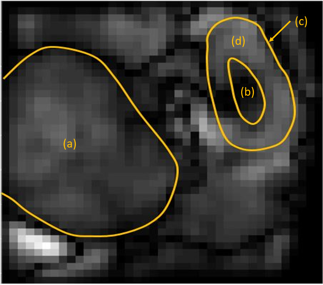
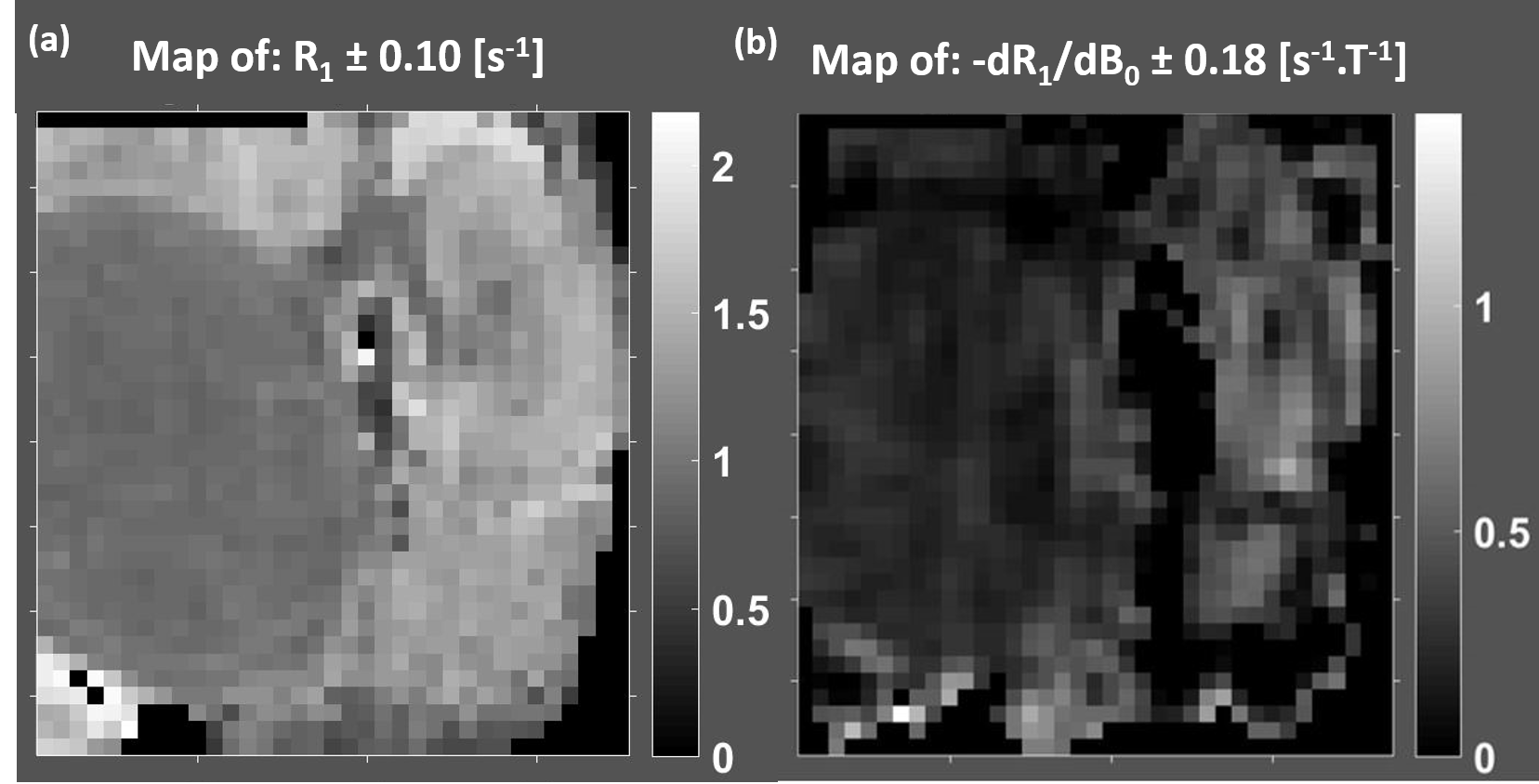
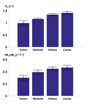
The TI=540 ms inversion image at 1.5T provided a good T1 contrast to identify the different kidney regions and the tumor (Fig.1). Uniform values for R1 and dispersion maps for the tumor (Fig.2) were obtained as well as differences between the medulla and the cortex (Fig.2). The tumor displayed lower R1 and dispersion than the medulla and the kidney (Fig.3). Considering the average values over the different regions of interest for all animals, a strong correlation (r=0.93) was observed between R1 and the dispersion.Discussion/Conclusion
In vivo measurements of R1-dispersion around 1.5 T have been performed in a kidney cancer model on 27 mice in a reproducible manner demonstrating stability of our unique FFC-MRI prototype. When averaged over a ROI, the slope of the NMRD profile could be used to differentiate tumors from healthy kidneys. The correlation of dispersion around 1.5T with R1 at 1.5 T suggests that both parameters bears the similar information. If normalized by R1, it seems that correlation is reduced suggesting that dispersion properties may provide an additional biomarker. Sensitivity could be increased by producing higher field shifts or by using dynamic sequence instead of inversion recovery. Further in vivo analysis are needed to investigate the differences in R1-dispersion among various tumor types and healthy tissue and its potential benefit among existing MR parameters at fixed B0 field.Acknowledgements
Study implemented on the 1.5T MRI platform (CNRS, Univ Paris-Sud, CEA) and partly funded by « France Life Imaging, grant ANR-11-INBS-0006 ».
Nephroblastoma samples available thanks to the MAPPYACTS project, Gustave Roussy.
References
[1] Lurie D.J., et al., C. R. Physique (2010);11 :136-148. [2] Alford, J.K., et al., Magn Reson Med (2009) 61:796–802. [3] Hoelscher, U.C., et al., Magn Reson Mater Phy (2013) 26:249–259. [4] Bödenler, M., et al., ESMRMB; 55 (2017). [5] Chanet N., et al., ESMRMB; 427 (2017). [6] De Rochefort L., et al., Proc. Intl. Soc. Mag. Reson. Med. 20, abstract 4165 (2012). [7] Chanet N., et al., Proc. Intl. Soc. Mag. Reson. Med. 25, abstract 3792 (2017).Figures