2252
A dual-step iterative temperature estimation method for accurate and precise fat referenced PRFS temperature mapping1Shenzhen Institutes of Advanced Technology, Chinese Academy of Sciences, Shenzhen, GuangDong, China, 2University of Chinese Academy of Sciences, Beijing, China
Synopsis
Temperature imaging based on proton resonance frequency shift (PRFS) fails in fat containing tissues as the proton frequency of fat does not change with temperature. A dual-step iterative temperature estimation of fat referenced PRFS method is proposed to improve both the accuracy and precision of fat-referenced PRFS method. The method is evaluated with fat-water phantom and ex vivo BAT tissue excised from rats. Compared to the existing methods, the proposed method has least bias to the fluorescent optical fiber thermometer while maintaining the best noise performance.
Introduction:
Temperature imaging based on proton resonance frequency shift (PRFS) fails in fat containing tissues as the proton frequency of fat does not change with temperature. Several groups has proposed fat-referenced PRFS methods to overcome this problem1,2. In these methods, resonance frequency difference between fat and water protons was considered as an unknown parameter in the signal model, and temperature change was obtained from the water-fat resonance frequency difference. However, the signal models adopted by these studies have been simplified. The accuracy of the temperature imaging was compromised. In the present study, a dual-step iterative temperature estimation of fat referenced PRFS method is proposed. The phantom and ex-vivo experiment shows the proposed method has least bias to the optical fiber thermometer while maintaining best noise performance compared to existing methods.Theory and methods:
The signal model of multi-echo data considering temperature change is formulated as follow:$$s_n=\left(A_We^{iΦ_W}e^{-i2πγB_0 αTE_nΔT}e^{-\frac{TE_n}{T_{2,W}^*}}+A_Fe^{iΦ_F}\sum_{p=1}^Pβ_pe^{-i2πγB_0 f_{F,p}TE_n}e^{-\frac{TE_n}{{T_{2,F}^*}}}\right)e^{-i2πf_BTE_n},n=1,2,3...,N(1)$$
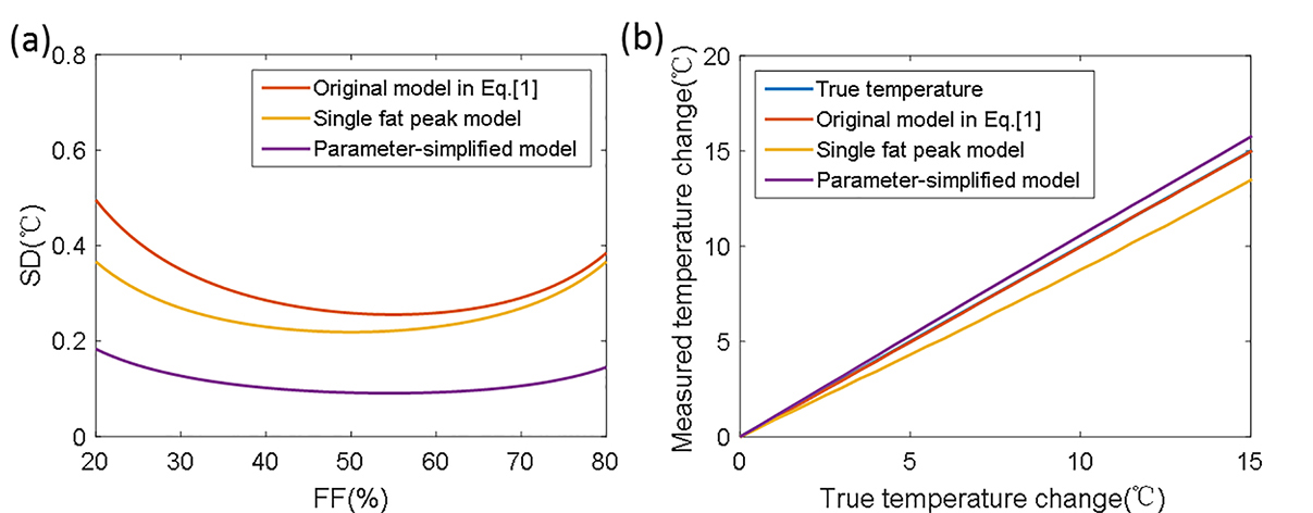
where α is the proton resonance frequency shift coefficient (typically, $$$α=-0.01 ppm/℃$$$), and ΔT is the temperature change from the baseline temperature. The fat component consists of P peaks with relative amplitudes $$$β_p$$$ and chemical shift $$$f_{F,p}$$$, and $$$∑_{p=1}^Pβ_p=1$$$. In this original model, eight unknown parameters $$$\left\{{A_W,Φ_W,T_{2,W}^*,A_F,Φ_F,T_{2,F}^*,f_B,ΔT}\right\}$$$need to be estimated. Li et al1 used single peak model of fat. Wyatt et al2 assumed $$$\left\{Φ_W,T_{2,W}^*,Φ_F,T_{2,F}^* \right\}$$$ were constant and only four parameters $$$\left\{A_W,A_F,f_B,ΔT\right\}$$$ were jointly estimated. Although the noise performance is improved with the decrease number of unknowns, as shown in Fig. 1a, the estimation is biased with time and temperature change ,as shown in Fig.1b. The overall performance of these methods based on the simplified models is therefore compromised.
We proposed a dual-step iterative temperature estimation algorithm to improve both the accuracy and precision of fat-referenced PRFS method. The steps for the dynamic temperature measurement are introduced as follows:
(1) The whole images are processed by a fat-water separation algorithm3 to solve the fat and water ambiguity first at an initial $$$ΔT$$$.
(2) The eight parameters $$$\left\{{A_W,Φ_W,T_{2,W}^*,A_F,Φ_F,T_{2,F}^*,f_B,ΔT}\right\}$$$ are obtained through nonlinear fitting to Eq.[1] using the results from (1) as initial values.
(3) After the nonlinear fitting in step (2) is done pixel-by-pixel in ROI, the temperature change map is smoothed by a spatial low pass filter.
(4) The seven parameters $$$\left\{A_W,Φ_W,T_{2,W}^*,A_F,Φ_F,T_{2,F}^*,f_B\right\}$$$ are re-fitted to Eq.[1] using the smoothed $$$ΔT$$$ as given value.
(5) The four parameters $$$\left\{A_W,A_F,f_B,ΔT\right\}$$$ are re-fitted to Eq.[1] using $$$\left\{Φ_W,T_{2,W}^*,Φ_F,T_{2,F}^* \right\}$$$ as given values.
(6) $$$ΔT$$$ at current measurement is used for the initial value for the next measurement.
To demonstrate the performance of the proposed method, experiments on fat-water phantoms and ex-vivo brown adipose tissue (BAT) were designed. The MRI scans were implemented on a 3T system (TIM TRIO, Siemens, Germany) with a six-echo FLASH sequence. The basic protocols were: TR=40ms, resolution=0.82×0.82mm2 (phantom)/0.69×0.69mm2 (BAT), slice thickness=10mm, flip angle=30°, TE1/ΔTE=6/6ms (phantom) and 6.53/1.9ms (BAT). The phantom/BAT was put in a water tank with the same temperature of scan room. For the heating experiment, the whole tank was immersed in a warmer water bath immediately before the scan and an optical fiber thermometer was inserted into the phantom/BAT to monitor the temperature change during the scan.
Results:
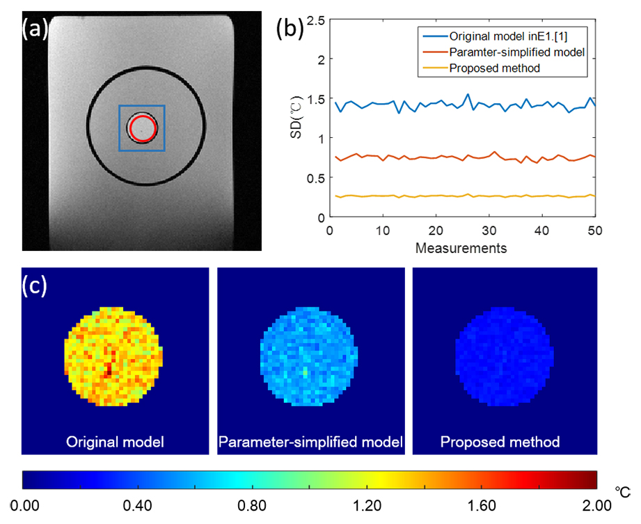
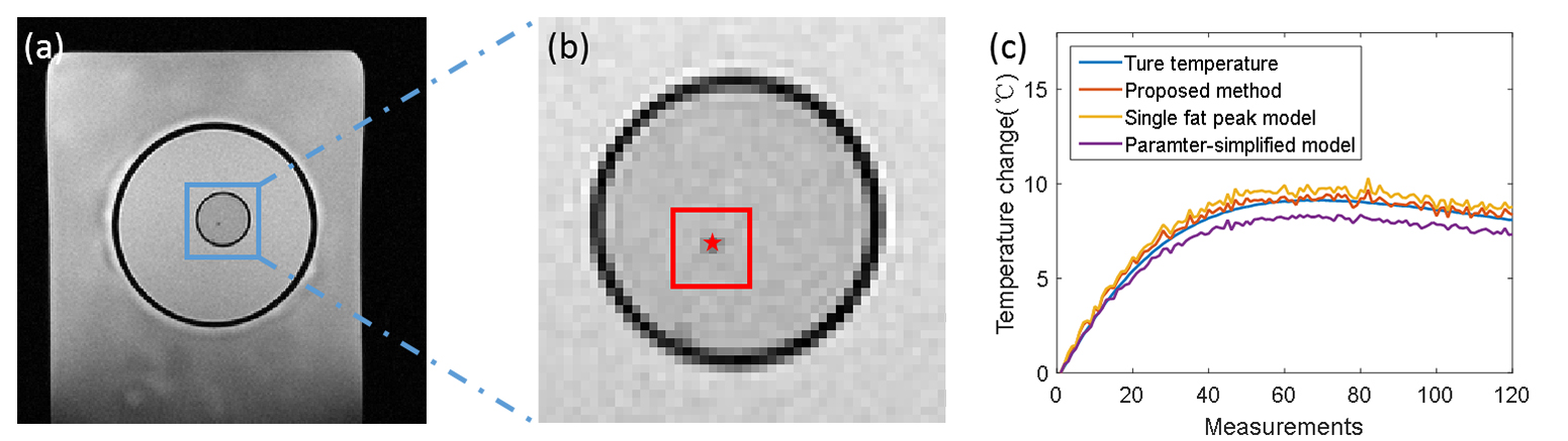
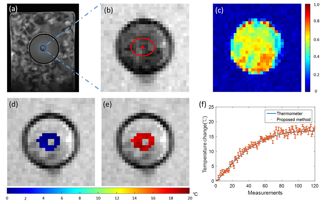
Figure 2 compares the temperature noise performance between the two simplified models and the proposed method in phantom experiment with invariant temperature. The proposed method had the lowest standard deviation (SD) of temperature change than the two simplified models. Figure 3 compares the results of phantom heating experiment between the two simplified models and the proposed method. It is shown that the mean temperatures obtaining by simplified models diverged from the true values from thermometer, while the proposed method shows little bias. Figure 4 shows the results of ex vivo BAT heating experiment. The temperatures by the proposed method was consistent with the values measured by thermometer with a small SD (min/mean/max SD=0.32/0.46/0.65 over all measurements) within ROI.Discussion and conclusions:
Although the noise performance of simplified signal models is better than original model, the model becomes biased due to change of parameters $$$\left\{Φ_W,T_{2,W}^*,Φ_F,T_{2,F}^* \right\}$$$ during the measurements. The initial phases vary slowly during the measurements due to system hardware performance fluctuation and the $$$T_2^*$$$ also change with temperature. The model with single fat peak introduces an extra nonlinear term between water and fat proton frequency which results in temperature error. The proposed method jointly estimates all eight unknown parameters with multiple fat peak model, which ensures the temperature estimation is unbiased. Meanwhile, the smoothness operation on temperature map restrains the variance of the phases and $$$T_2^*$$$ of water and fat, which can be attributed to the improvement of noise performance of temperature estimation in the proposed method.Acknowledgements
This research was supported by the National Natural Science Foundation of China No. 81327801, 61302040,11504401, 81527901, 81301242, U1301258, National Key R&D Program No. 2016YFC0100100, Shenzhen Scienceand Technology Research Program No. JCYJ20150630114942317 and JCYJ20150521094519487
References
1. Li C, Pan X, Ying K, et al. An internal reference model-based PRF temperature mapping method with Cramer-Rao lower bound noise performance analysis[J]. Magn Reson Med, 2009, 62(5): 1251-1260.
2. Wyatt C, Soher B J, Arunachalam K, et al. Comprehensive analysis of the Cramer–Rao bounds for magnetic resonance temperature change measurement in fat–water voxels using multi-echo imaging[J]. Magn. Reson. Mater. Phys., Biol. Med., 2012, 25(1): 49-61.
3. Cheng C, Zou C, Liang C, et al. Fat-water separation using a region-growing algorithm with self-feeding phasor estimation[J]. Magn Reson Med, 2017, 77(6): 2390-2401.
Figures