2246
Comparison between static and dynamic B0-mapping methods for accurate frequency correction of CEST in the presence of temporarily fluctuating B0 inhomogeneities at 7T1Biomedical Imaging and Image-guided Therapy, Medical University of Vienna, Vienna, Austria, 2Christian Doppler Laboratory for Clinical Molecular MR Imaging, Vienna, Austria, 3Department of Physics, University of Helsinki, Helsinki, Finland
Synopsis
Chemical Exchange Saturation Transfer is prone to inhomogeneities of the static magnetic field (B0). Hence, accurate frequency correction is mandatory for reliable quantification. Currently established B0 correction approaches assume B0 inhomogeneities to be static during CEST experiments, but this is questionable in the presence of subject motion and scanner instabilities. Thus, we propose three different dynamic B0 correction methods for CEST that can compensate for B0 instability for each Z-spectral point separately and compare them to three established static B0 correction approaches that apply the same frequency shift to all Z-spectral points in phantom and in vivo experiments.
INTRODUCTION
Chemical Exchange Saturation Transfer(CEST) imaging benefits from ultra-high-field MR due to increased spectral resolution, but it is also prone to B0 inhomogeneities, which are increasing at higher B0. Corrections are required in particular when investigating Z-spectra close to water[1]. Current CEST data processing techniques assume stable B0 conditions during the measurement, thus applying the same shift to each off-resonance irradiation frequency. These approaches cannot compensate for inevitable temporal B0 changes during a CEST experiment. Here we propose three different dynamic B0 correction methods for CEST that can compensate for B0 instability for each Z-spectral point separately and compare them to three established static B0 correction approaches that apply the same frequency shift to all Z-spectral points.MATERIALS AND METHODS
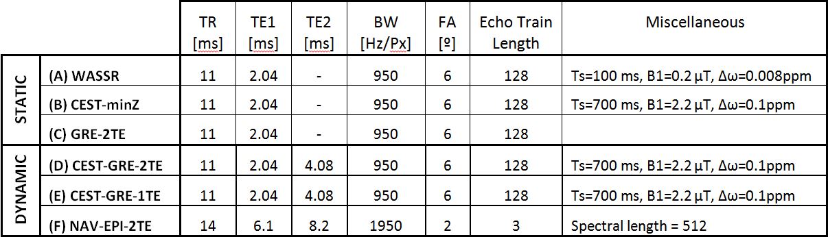
The three static B0 acquisition approaches were:
(A)WASSR: Water frequency from the central value of a Z-spectrum with high spectral resolution and low saturation power(=prescan)[1]
(B)CEST-minZ: Water frequency from the minimum value of the interpolated Z-spectra itself(=intrinsic)[2]
(C)GRE-2TE: B0 shift map from a dual-echo gradient echo readout reference scan, acquired before the CEST sequence(=prescan)[3]
The three dynamic B0 correction approaches were:
(D)CEST-GRE-2TE: B0 maps from a dual-echo gradient echo CEST readout (after RF saturation)(=intrinsic).
(E)CEST-GRE-1TE: The same as (D) but with a single-echo readout. A reference scan (C) is required initially to determine coil offset maps(=intrinsic/prescan)[4]
(F)NAV-EPI-2TE: B0 maps from a dual-echo multi-shot EPI readout from a navigator interleaved within the CEST scan(=interleaved)[5]
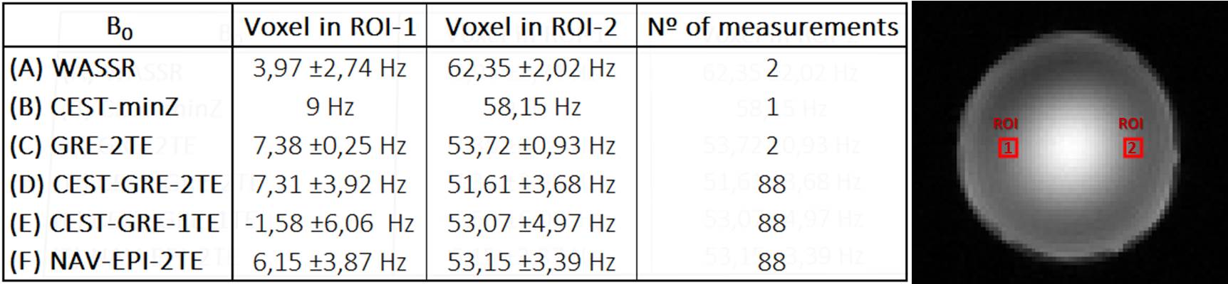
To evaluate the precision measuring the effective applied off-resonance frequencies, a phantom containing no Magnetization Transfer(MT) or chemical exchange was used. The closest the MTRasym to 0, the more precise is the method.
All the scans where performed on a whole-body 7T MR system (Siemens, Erlangen, Germany) with a 1H 32-channel head coil. Phantom scans were carried out on a cylindrical 0.5L plastic bottle with a 0.5 mM Manganese chloride solution and gadolinium contrast agent to match T1/T2 of grey matter in-vivo at 7T.
In phantoms, a linear B0 gradient in the readout encoding direction was induced and differences between static and dynamic correction were evaluated (Table.2).
To show the performance of dynamic compensation methods versus the static ones in the presence of scanner instabilities, a linear frequency drift of 60Hz was induced while scanning a healthy volunteer.
CEST saturation trains consisted of four 100ms Gaussian pulses, 50% duty cycle, B1rms=2.2uT, Z-spectra range ±4.5ppm, step size 0.1ppm (87/91 saturation offsets + normalization for phantom/in vivo), alternating between positive to negative offsets.
Image acquisition parameters were matched whenever possible for all the methods(A-F, see details Table 1) with a resolution of 1.7x1.7x6.0mm³, FOV=220x220mm²(phantom) and 2x2x6mm³, FOV=260x260mm²(in-vivo). WASSR images were obtain with the same parameters as CEST, but only one saturation pulse of B1rms=0.2uT within ±1.0ppm(step size 0.008 ppm).
RESULTS AND DISCUSSION
Tab.2 show that all B0 mapping approaches provided reproducible frequency estimation with variability ranging from 0.25Hz to ~6Hz. Frequency accuracy was in the range of a -2% to 7%. Among the dynamic approaches temporal variability was lowest for (D)CEST-GRE-2TE and (F)NAV-EPI-2TE and highest for (E)CEST-GRE-1TE.
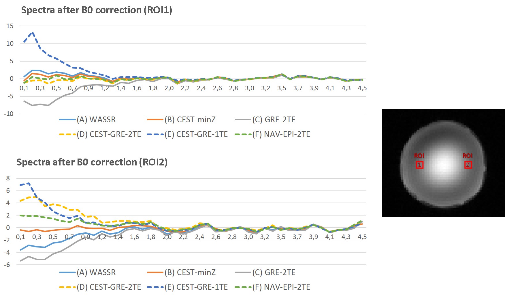
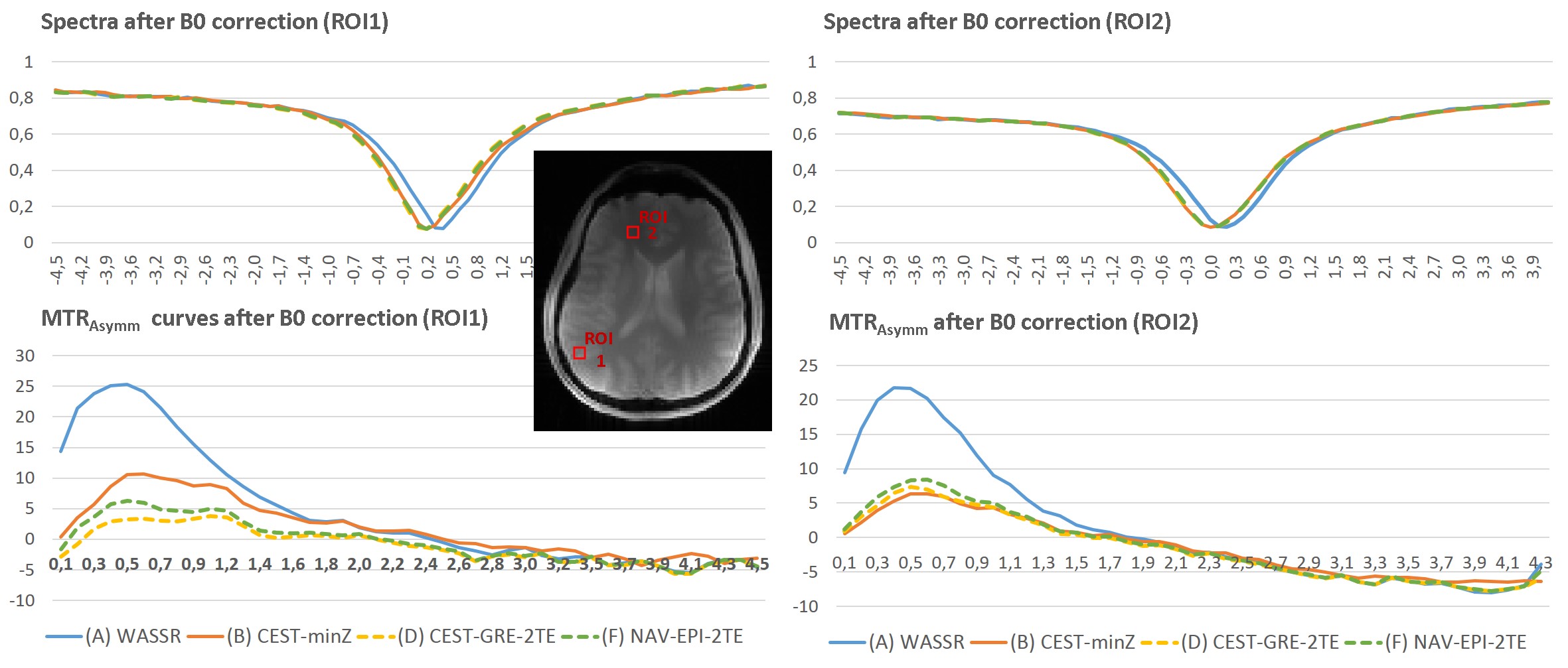
The effects of B0 corrections on MTR asymmetry curves are shown in Fig.1 as averages of the voxels contained in the same two ROI presented in Tab.1.
In the water phantom, where no MT and CEST effects are expected, (B)CEST-minZ performed best among all static approaches, while (C)GRE-2TE seems to create an artificial negative peak for resonances <1.6ppm (too low B0 was calculated).
Among all dynamic method only B0 estimation by (F)Nav-EPI-2TE was completely insensitive to CEST contrast changes for labeling at <1.2ppm. For >1.2ppm (D)CEST-GRE-2TE and (E)CEST-GRE-1TE provided better results.
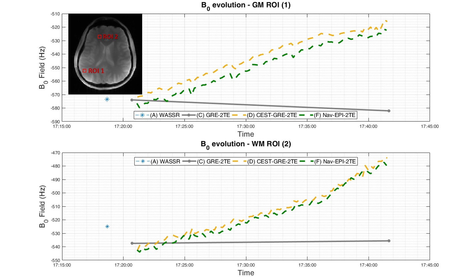
Preliminary in vivo results (Fig.2) show how accurately (D)CEST-GRE-2TE and (F)Nav-EPI-2TE tracked the linear frequency drift of 60Hz, which cannot be taken into account using static approaches (A-C).
A 60Hz drift over 90 measurements in ROI1 translated to 0.67Hz/measurement, which is consistent with the assessment by (D)CEST-GRE-2TE 0.62Hz/measurement(95%-CI:0.60-0.64; R2=0.98) and (F)Nav-EPI-2TE 0.64Hz/measurement(95%-CI:0.60-0.64; R2=0.99).
In contrast, using the static correction (A)WASSR the minimum of Z-spectra is shifted≈60Hz(0.2ppm) from water creating a positive artificial peak ~0.4ppm of amplitude greater than 20%(Fig.3). (B)CEST-minZ is able to reduce this effect down to 6-10%, because the correction in (B) is based on data acquired after ~60Hz drift, but (A) when no drift was present at the beginning.
The dynamic methods (D)CEST-GRE-2TE and (F)Nav-EPI-2TE generate similar MTR asymmetry curves after correction, but with a slightly higher peak at ~0.5ppm for (F).
CONCLUSIONS
This
study shows the benefits of using intrinsically obtained B0 maps
during a CEST experiment to perform dynamic frequency correction of each
individual Z-spectral point in the presence of temporarily fluctuating B0-inhomogeneities.
This will be another important step towards reliable CEST imaging for clinical
use.Acknowledgements
We would like to thank the Christian Doppler Laboratory for Clinical Molecular MR Imaging, Vienna, Austria for their financial support of this study.References
1. Kim, M., et al., Water saturation shift referencing (WASSR) for chemical exchange saturation transfer (CEST) experiments. Magn Reson Med, 2009. 61(6): p. 1441-1450.
2. Zaiss, M., B. Schmitt, and P. Bachert, Quantitative separation of CEST effect from magnetization transfer and spillover effects by Lorentzian-line-fit analysis of z-spectra. J Magn Reson, 2011. 211(2): p. 149-155.
3. Kawanaka, A. and M. Takagi, Estimation of static magnetic field and gradient fields from NMR image. Journal of Physics E: Scientific Instruments, 1986. 19(10): p. 871.
4. Robinson, S., et al., Combining phase images from multi-channel RF coils using 3D phase offset maps derived from a dual-echo scan. Magn Reson Med, 2011. 65(6): p. 1638-1648.
5. Bogner W, et al., Real-time motion- and B0-correction for LASER-localized spiral-accelerated 3D-MRSI of the brain at 3T. Neuroimage. 2014 Mar;88:22-31. doi: 10.1016/j.neuroimage.2013.09.034. Epub 2013 Nov 5.
Figures