2216
Fast brain iron quantification using QSM with low spatial resolution1Biomedical Engineering, University of Southern California, Los Angeles, CA, United States, 2Ming Hsieh Department of Electrical Engineering, University of Southern California, Los Angeles, CA, United States, 3Cardiology, Children's Hospital Los Angeles, Los Angeles, CA, United States
Synopsis
This study investigates the impact of spatial resolution on QSM susceptibility mapping for brain iron quantification. We obtained 40 sub-millimeter resolution whole-brain QSM datasets, and simulated six levels of spatial resolution via k-space truncation. QSM-based iron quantification was performed at each spatial scale and compared against the reference. We found that estimation error was ≤ 5 ppb in the basal ganglia when the voxel dimension along all three axes was ≤ 2.0 mm. The finding suggests that scan time can be significantly shortened by reducing spatial resolution.
Introduction
Recent research has uncovered a relationship between iron overload in the basal ganglia and neurodegenerative diseases1. The congregation of non-heme iron in the basal ganglia creates strong signal detectable in QSM images. We see QSM to be a promising tool to measure the concentration of iron in those regions2-5. Current QSM protocols serve several purposes and require long scan times (4-10 minutes) due to the use of long echo times, broad spatial coverage, and submillimeter spatial resolution. We now know that long echo times and broad spatial coverage are critical to the sensitivity and accuracy of susceptibility measurement4,5. This study investigates the importance of spatial resolution on the quantification of brain iron. We retrospectively truncated raw k-space data from 40 sub-millimeter resolution QSM in-vivo datasets to simulate lower resolution acquisitions. Iron quantification in the basal ganglia was performed at each spatial scale and compared against the reference fully sampled data.Methods
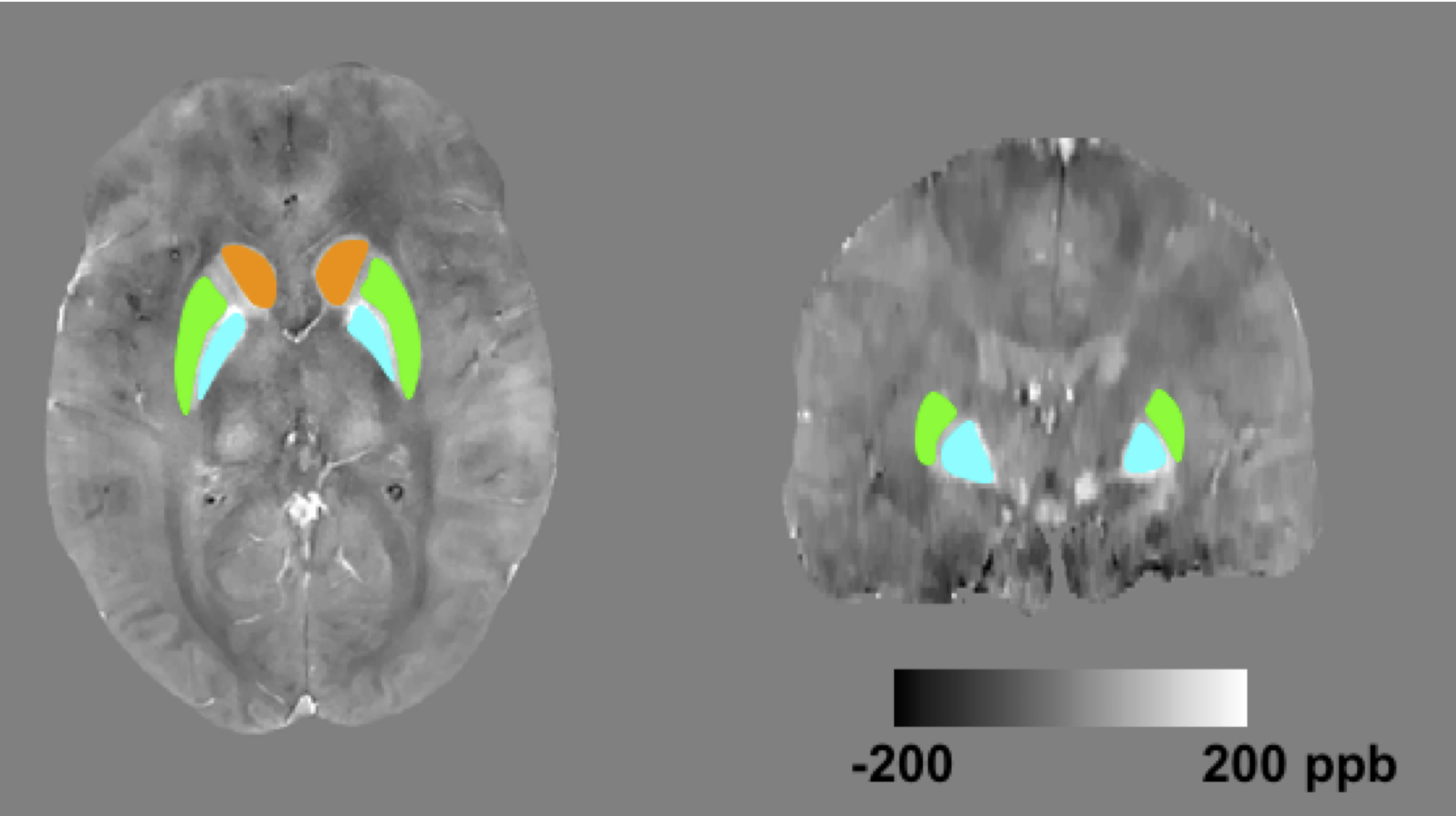
Datasets: 20 healthy subjects and 20 anemia patients (15 men, 25 women; age, 24±8 years old) were scanned using a 3D multi-echo gradient echo sequence on the Philips 3T Achieva system with a 32-channel head coil. Acquisition parameters: spatial resolution= 0.6x0.6x1.3 mm3, FOV = 22x22x12 cm3, TE=5:5:20 ms, TR=40 ms. Written informed consent was obtained, and the protocol was approved by our Institutional Review Board. Simulation: Six levels of spatial resolution were simulated by truncating the acquired data in k-space. Before QSM processing, all datasets were zero-padded to have the same matrix size as the reference data. B0 field was computed by fitting the multi-echo phase images. Laplacian phase unwrapping was performed6. Background field was removed using project onto dipole field (PDF)7. Unreliable phase points were excluded3. L1-norm constrained reconstruction2 was used to derive susceptibility map from local B0 field (λ= 4x10⁻⁴). Evaluation: 3D ROI masks for the caudate nucleus (CN), putamen (PT) and globus pallidus (GP) were defined based on T1-weighted images, and registered to the QSM datasets. Figure 1 shows the segmentation of the three ROIs in both axial and coronal views. At each spatial scale, average susceptibility within the ROI was computed and compared against the reference. Error was computed as $$$\hat \chi-\chi_{ref}$$$, where $$$\hat \chi$$$ and $$$\chi_{ref}$$$ are the intra-ROI average susceptibility in the low-resolution and the reference data respectively. One-sample student t-test was performed on measurement error.Results
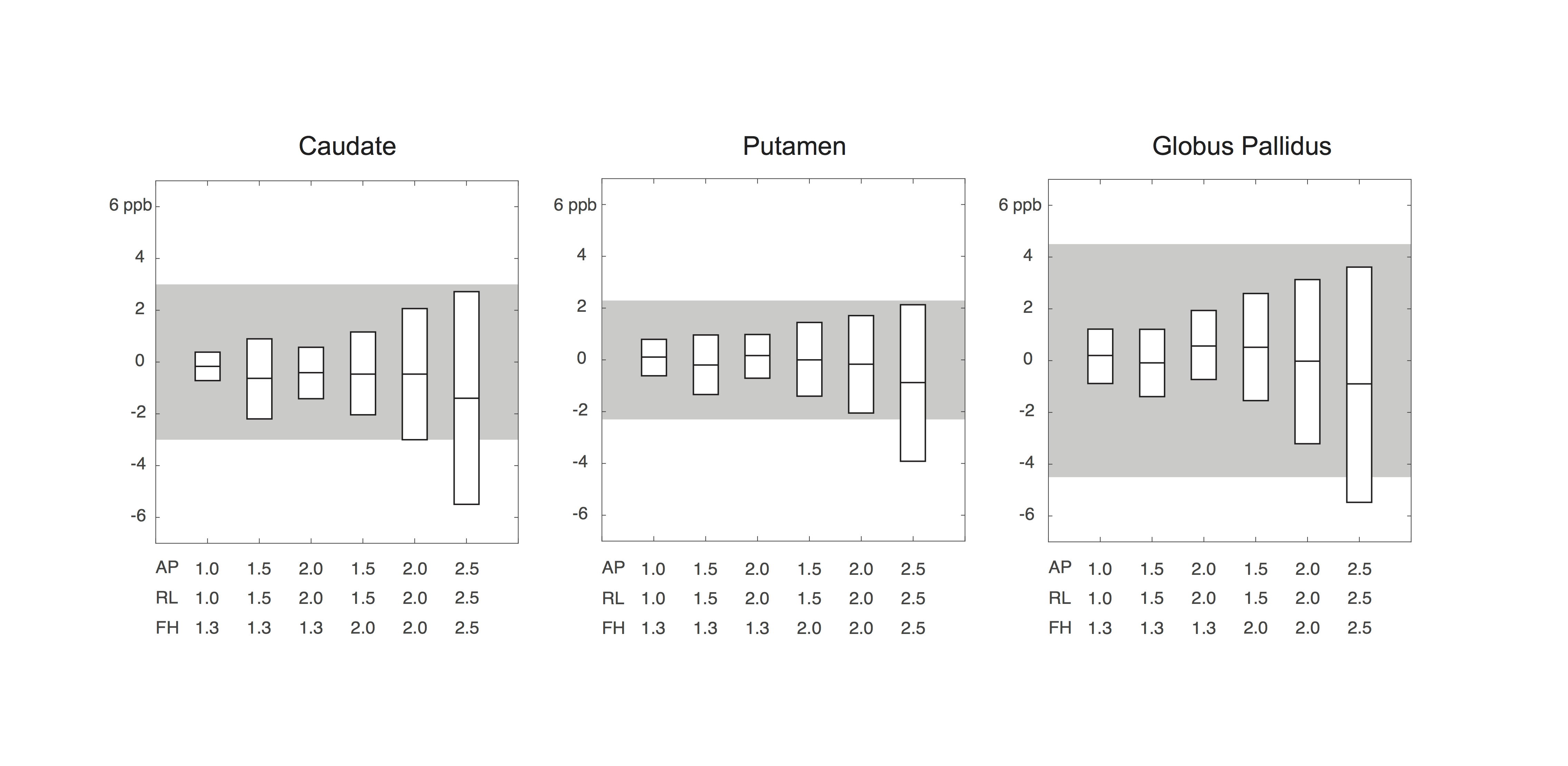
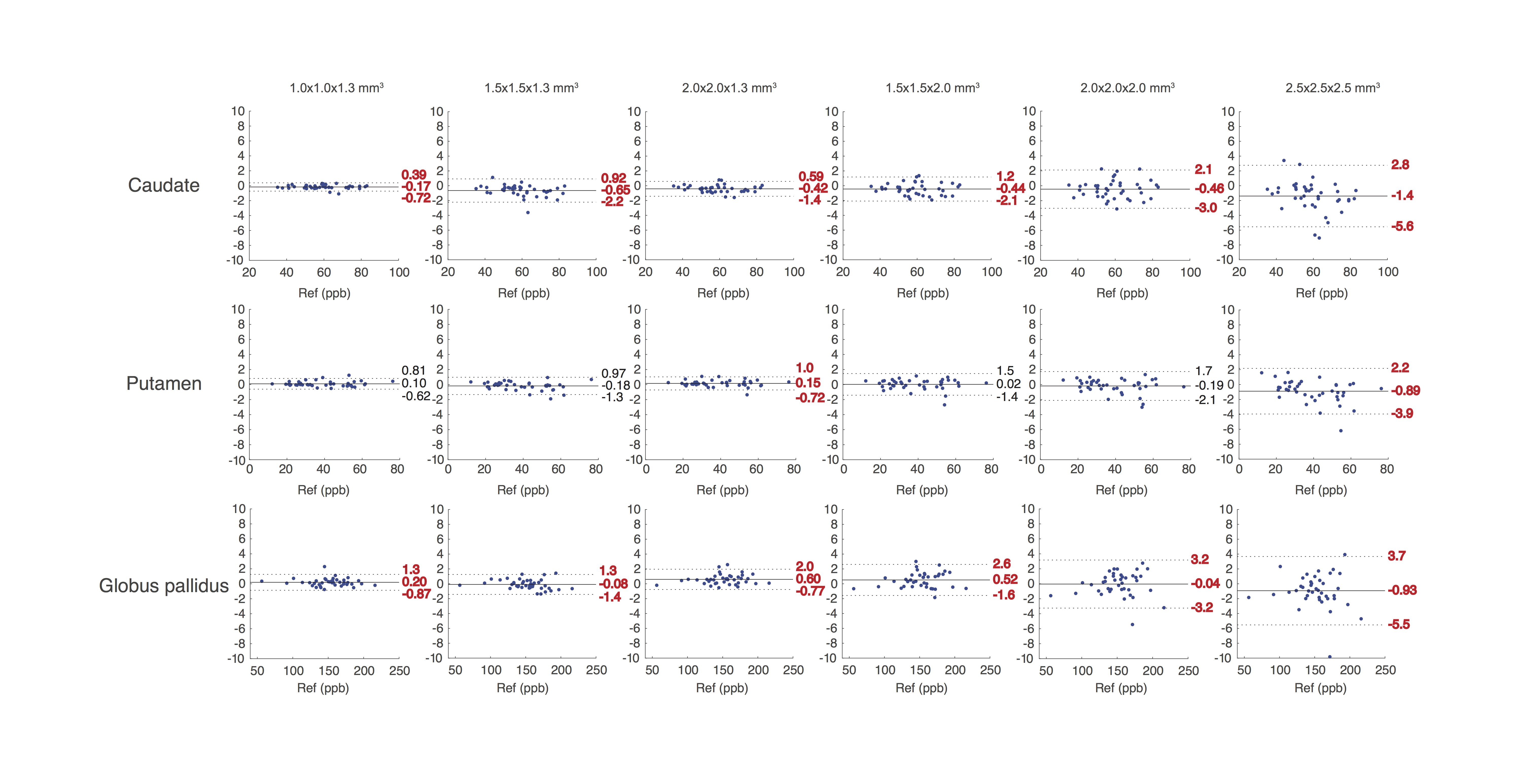
Figure 2 summarizes the error of susceptibility measurement (in parts per billion, ppb) at each level of spatial resolution. The boxes represent the 95% confidence interval (i.e. mean±2.03SD) of the mean measurement error. The range of acceptable error (±5 ppb) was denoted as gray area. Estimation error was ≤ 5 ppb in all three regions, when the voxel dimension along all three axes was ≤ 2.0 mm. Figure 3 is the Bland-Altman plot showing the error of susceptibility estimation against the reference at each spatial resolution. Significant measurement bias (p<0.05, t-test) was labeled in red. The bias was ≤ 0.65 ppb when the voxel dimension along all three axes was ≤ 2.0 mm.Discussion
This study evaluated the effect of spatial resolution on brain iron quantification using QSM. Through simulation on 40 in-vivo datasets, we found that susceptibility estimation error was below 5 ppb for the caudate, putamen and globus pallidus, when the voxel dimension along all three axes was ≤ 2.0 mm. Resolution in most QSM protocols has been largely motivated by a phantom study by Zhou et al.8, using Gadolinium contrast. The study showed 170 ppb (40%) susceptibility underestimation at 1.8 mm3 spatial resolution, 1.5T. Our experimental finding contradicts this prediction, likely because the prior study 1) involved a very high susceptibility, 400 ppb, more than twice what is typically encountered in basal ganglia nuclei, and 2) produced very high magnitude signal due to the use of T1-shortening contrast agent (4 times higher than the background), whereas susceptibility in brain tissue lowers the magnitude signal.
In recent literature on the repeatability of brain QSM9-11, Lin et al.9 and Santin et al.10 showed within-site variance of about 5 ppb in deep gray matter nuclei; Deh et al.11 showed a within-site variance above 12 ppb. In this study, we used 5 ppb as an acceptance threshold of measurement error. However, more study is needed to determine the clinical significance of such susceptibility measurement error in the basal ganglia. When brain tissue iron (not vascular) is the target of a QSM study, our findings indicate an opportunity to significantly shorten scan time by simply lowering spatial resolution.
Acknowledgements
This work is supported by the National Heart Lung and Blood Institute (1U01HL117718-01).References
1. Ward RJ, Zucca FA, Duyn JH, Crichton RR, Zecca L. The role of iron in brain ageing and neurodegenerative disorders. Lancet Neurol. 2014;13(10):1045-1060.
2. Bilgic B, Pfefferbaum A, Rohlfing T, Sullivan E V., Adalsteinsson E. MRI estimates of brain iron concentration in normal aging using quantitative susceptibility mapping. Neuroimage. 2012;59(3):2625-2635.
3. Schweser F, Deistung A, Lehr BW, Reichenbach JR. Quantitative imaging of intrinsic magnetic tissue properties using MRI signal phase: an approach to in vivo brain iron metabolism?. Neuroimage. 2011 Feb 14;54(4):2789-807.
4. Wang Y, Liu T. Quantitative susceptibility mapping (QSM): Decoding MRI data for a tissue magnetic biomarker. Magn Reson Med. 2015;73(1):82-101.
5. Haacke EM, Liu S, Buch S, Zheng W, Wu D, Ye Y. Quantitative susceptibility mapping: current status and future directions. Magn Reson Imaging. 2015;33(1):1-25.
6. Schofield MA, Zhu Y. Fast phase unwrapping algorithm for interferometric applications. Opt Lett. 2003;28(14):1194.
7. Liu T, Khalidov I, de Rochefort L, et al. A novel background field removal method for MRI using projection onto dipole fields (PDF). NMR Biomed. 2011;24(9):1129-1136.
8. Zhou D, Cho J, Zhang J, Spincemaille P, Wang Y. Susceptibility underestimation in a high-susceptibility phantom: Dependence on imaging resolution, magnitude contrast, and other parameters. Magn Reson Med. 2017;78(3):1080-1086.
9. Lin P-Y, Chao T-C, Wu M-L. Quantitative susceptibility mapping of human brain at 3T: a multisite reproducibility study. AJNR Am J Neuroradiol. 2015;36(3):467-474.
10. Santin MD, Didier M, Valabrègue R, et al. Reproducibility of R2* and quantitative susceptibility mapping (QSM) reconstruction methods in the basal ganglia of healthy subjects. NMR in biomedicine. 2017 Apr 1;30(4).
11. Deh K, Nguyen TD, Eskreis-Winkler S, et al. Reproducibility of quantitative susceptibility mapping in the brain at two field strengths from two vendors. J Magn Reson Imaging. 2015;42(6):1592-1600.
Figures