2205
Suitable image quality measures to evaluate quantitative susceptibility maps1Medical Physics in Radiology, German Cancer Research Center (DKFZ), Heidelberg, Germany
Synopsis
The 2016 QSM Reconstruction Challenge urged the need for a suitable quality measure of susceptibility maps as classical image quality measures (root-mean-square error, high-frequency error-norm, structural similarity index) were no suitable indicators of the visual quality of susceptibility maps. Errors (noise, smoothing, streaking) were added to a reference susceptibility map and the sharpness-index-weighted structural similarity index was used to evaluate the degraded quantitative susceptibility maps and to compare the result with classical image quality measures. The sharpness-index-weighted structural similarity index was shown to be a suitable measure for QSM image quality with a strong devaluation of over-smoothed images.
Introduction
The QSM algorithms tested in the 2016 QSM Reconstruction Challenge (1) were optimized to minimize image quality measures. As a result the obtained susceptibility maps showed over-smoothing effects and a notable loss of details. Therefore, the challenge highlighted the need for a suitable image quality measure. The purpose of this work is to solve this problem by applying an image quality criterion which effectively devaluates over-smoothing.
Theory
The structural similarity index (SSIM) (2) was developed to assess perceptual image quality of a distorted image relative to a reference image. The sharpness index (SI) (3, 4) was derived for its use in image processing and in image quality assessment.
Let $$$\Omega=\mathbb{Z}^2\cap\left(\left[-\frac{M}{2}\right) \times\left[-\frac{N}{2},\frac{N}{2}\right)\right)$$$ be the rectangular image domain and $$$u:\Omega\to \mathbb{R}$$$ a gray-level image. The image gradient is then defined as $$\nabla u(x,y)=\left(\begin{array}{c}\partial_x \dot{u}(x,y)\\ \partial_y\dot{u}(x,y)\end{array}\right)=\left(\begin{array}{c}\dot{u }(x+1,y)-\dot{u}(x,y)\\\dot{u}(x,y+1)-\dot{u}(x,y)\end{array}\right)$$ Here $$$\dot{u}$$$ is the periodic extension of $$$u$$$. The Total Variation (TV) of $$$u$$$, given by $$\text{TV}(u)=\sum_{x\in\Omega} |\partial_x\dot{u}(\textbf{x})|+|\partial_y\dot{u}(\textbf{x})|,$$ measures how strong the function $$$\dot{u}$$$ oscillates. The sharpness index of an image $$$u$$$ is defined as $$\text{SI}(u)\equiv-log_{10}\phi\left(\frac{\text{TV}(u)-\mu}{\sigma}\right)$$ Here $$$\phi(t)\equiv\frac{1}{\sqrt{2\pi}}\int_{-\infty}^te^{-\frac{s^2}{2}}ds$$$ for $$$t\in\mathbb{R}$$$ is the Gaussian normal distribution, $$$\mu=\mathbb{E}(\text{TV}(u\ast W)),\quad\sigma^2=\mathbb{V}ar(\text{TV}(u\ast W)),$$$ and $$$W$$$ is Gaussian white noise with standard deviation $$$|\Omega|^{-\frac{1}{2}}$$$.
This means, the higher the SI, the smaller the probability for TV to decrease by randomization of u. Intuitively, for a sharp image the probability that the randomized image has a smaller TV is very small, leading to a high SI. For a blurred image this probability is higher and therefor SI lower.
The structural similarity index for a degraded image $$$u_{deg}$$$ relative to a reference image $$$u_{ref}$$$ is calculated as $$\text{SSIM}(u_{deg},u_{ref})\equiv[l(u_{deg},u_{ref})]^\alpha [c(u_{deg},u_{ref})]^\beta[s(u_{deg},u_{ref})]^\gamma$$ The function $$$l,c,s$$$ compare the luminance, contrast and structure information of the images. $$$\alpha,\beta,\gamma$$$ are parameters for adjustment. In practice the SSIM index is calculated locally and the mean value is used to quantify the overall image quality.
The sharpness index weighted SSIM (SI-SSIM ) (4, 5) is then defined as:$$\text{SI-SSIM}\equiv\begin{cases}\text{SSIM}\frac{\text{SI}(u_{deg})}{\text{SI}(u_{ref})},&\text{SI}(u_{deg})\leq \text{SI}(u_{ref})\\\text{SSIM},&\text{SI}(u_{deg})>\text{SI}(u_{ref}).\end{cases}$$
Methods
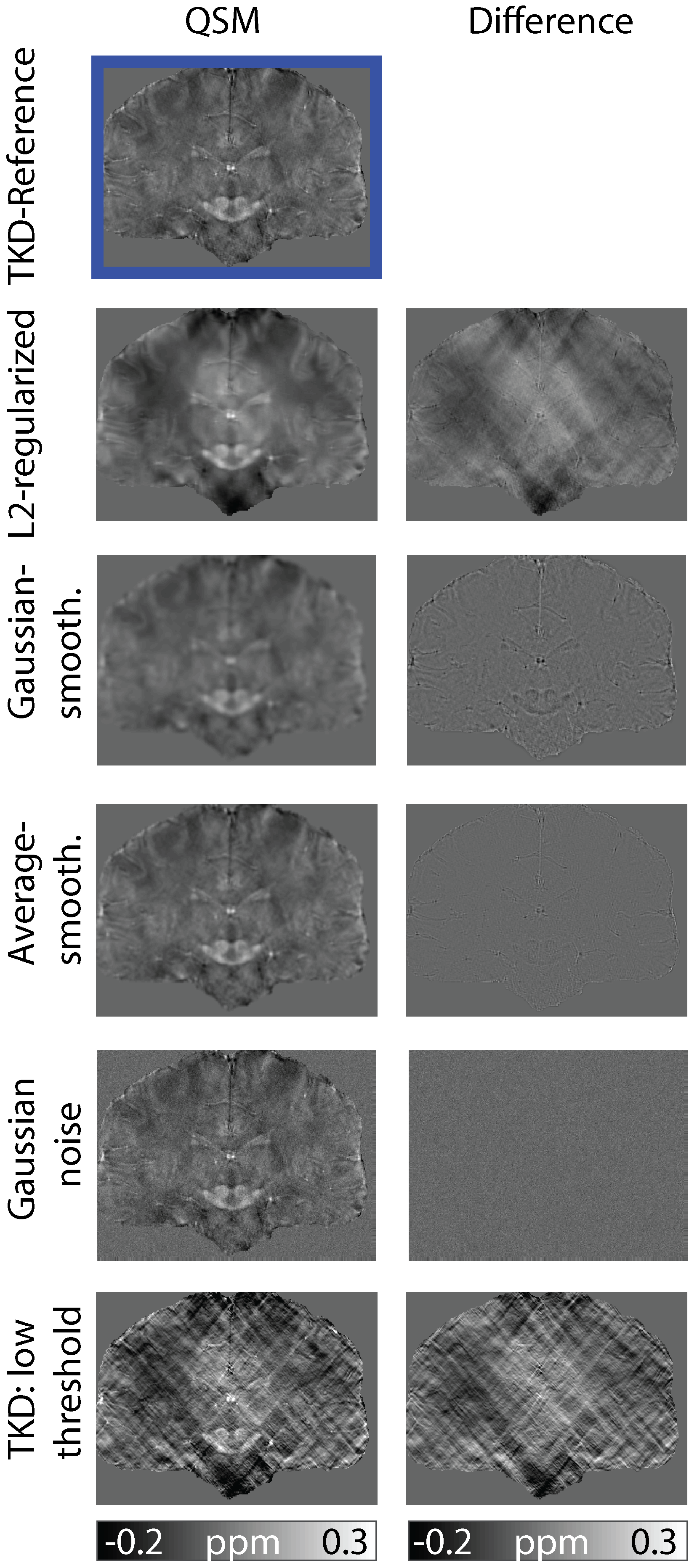
For the analysis we used gradient-echo phase data acquired at 7 Tesla with 0.5 mm isotropic resolution. Image analysis was done with Matlab, starting from background field corrected, unwrapped phase data. As QSM reconstructions we applied threshold-based k-space division (TKD) (6) and a closed-form L2-regularized algorithm (7). The TKD reconstructed image was assumed to be the ground truth to which we added several errors: Filtering with a 2-D Gaussian smoothing kernel with standard deviation 2 and with an averaging filter of size [3, 3]. Further, we added Gaussian white noise of mean 0 and variance 0.001, and we considered a TKD reconstructed image with a very low k-space threshold (0.03 compared with 0.19 for the ground truth), such that the image was contaminated by strong streaking artifacts (8). Deviations from the TKD reference map were quantified using the following image quality measures: root-mean squared error (RMSE), high-frequency error norm (HFEN), structure similarity index and the Sharpness Index weighted SSIM. To compute the SSIM we used the Matlab ssim-function with default settings as well as the implementation used in the reconstruction challenge. To compute the SI-SSIM, we used the implementation of the SI downloadable from (9).Results & Discussion
Figure 1 displays in the first column the susceptibility maps obtained by the different reconstruction algorithms and the degraded images. In the second column, the difference of these images to the reference image is shown.
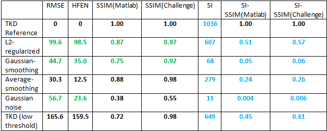
Table 1 lists the different image quality measures for the images
shown in Figure 1. The classical image quality measures are not very sensitive to
over-smoothing and noise effects. Only the structural similarity index seems to
detect noise. The image with streaking artifacts is also not highly devaluated by those measures. Furthermore, the Matlab-ssim function with default settings seems
to be a little improvement compared to the implementation used in the
reconstruction challenge.
The sharpness index highly devaluates the over-smoothed images as well as the image with additional noise. It is also sensitive to the streaking artifacts and the L2-reconstruction. This is in good accordance with the visual perception. These lower values of the sharpness index result in an overall and partially strong decrease from the SIMM value down to the SI-SIMM value: The SI-SSIM value for the Gaussian smoothed image is about one order of magnitude lower than the SI-SSIM value of the image obtained by the L2-regularized-reconstruction. The image with noise is even stronger devaluated.
Conclusion
The sharpness index seems to be a suitable measure to detect over-smoothing and noise effects. The resulting SI-SSIM, while maintaining the image quality measure properties of the structural similarity index, effectively devaluates images contaminated with such errors.Acknowledgements
This work was supported by a grant from Deutsche Forschungsgemeinschaft (Grant number: DFG STR 1480/2-1).References
1. Langkammer C. et al., Quantitative Susceptibility Mapping: Report from the 2016 Reconstruction Challenge. Magnetic Resonance in Medicine 2017; 00:00–00.
2. Wang Z. et al., Image Quality Assessment: From Error Measurement to Structural Similarity. IEEE Transactions on Image Processing January 2004; Vol. 13, No.1.
3. Gwendoline Blanchet, Lionel Moisan. An explicit Sharpness Index related to Global Phase Coherence. MAP5 2011-33. 2011.〈hal-00662374〉
4. Arthur Leclaire, Lionel Moisan. No-reference image quality assessment and blind deblurring with sharpness metrics exploiting Fourier phase information. Journal of Mathematical Imaging and Vision May 2015; Volume 52 Issue 1, pp 145–172.
5. Wang D., Ding W., Man Y., Cui L. A Joint Image Quality Assessment Method Based on Global Phase Coherence and Structural Similarity. 3rd International Congress on Image and Signal Processing 2010; (CISP2010)
6. Wharton S., Schäfer A., Bowtell R., Susceptibility mapping in the human brain using threshold-based k-space division. Magnetic Resonance in Medicine 2010; 63:1292–1304.
7. Bilgic B. et al., Fast Image Reconstruction With L2-Regularization. Journal of magnetic resonance imaging 2014; 40:181–191.
8. Li W et al., A method for estimating and removing streaking artifacts in quantitative susceptibility mapping. Neuroimage 2015; 108:111-122.
9. Moisan L., Sharpness Index. http://www.math-info.univ-paris5.fr/~moisan/sharpness/; called at 06.11.2017.
Figures