2202
Weak-harmonic regularization for quantitative susceptibility mapping (WH-QSM)1Department of Electrical Engineering, Pontificia Universidad Catolica de Chile, Santiago, Chile, 2Biomedical Imaging Center, Pontificia Universidad Catolica de Chile, Santiago, Chile, 3Martinos Center for Biomedical Imaging, Harvard Medical School, Charlestown, MA, United States, 4Department of Neurology, Medical University of Graz, Graz, Austria, 5Wellcome Centre for Human Neuroimaging, UCL Institute of Neurology, University College London, London, United Kingdom
Synopsis
In the context of QSM, the background pre-filtering step often leaves remnants in the local field, particularly in the vicinity of
Purpose
Since phase offsets in gradient-recalled echo (GRE) acquisitions are proportional to offsets in the main magnetic field, we can interpret the observed signal phase as a composite of two components. First, field inhomogeneities generated by imperfect shimming and magnetization sources outside the field of view, and second, the local phase resulting from the self-magnetization of the object of interest. In QSM, the latter, i.e. the local phase, is injected into an inversion routine to reconstruct the underlying tissue susceptibility distribution. Thus, external field contributions are often removed by dedicated algorithms prior to inversion to improve robustness. Notably, however, the resulting “local” phase often has remnants or artifacts from this step. On the observation that this is a common occurrence, we developed a regularized inversion method with a prior based on the harmonic property of the external field1,2 with the view to provide an additional layer of residual background filtering, which we hypothesized would lead to more accurate susceptibility reconstructions.Methods
The acquired phase within a given ROI is composed of local phase offsets and “external” contributions, which must be harmonic functions that satisfy Laplace’s equation1-3. A nonlinear functional with weak-harmonic regularization is then defined as: $$$argmin_{\chi,\phi_h}\frac{1}{2}\parallel w(e^{i(F^HDF\chi+\phi_h)}-e^{i\Phi}\parallel^2_2+\frac{\beta}{2}\parallel m\nabla^2\phi_h\parallel^2_2+R(\chi)$$$, with D the dipole kernel, χ the susceptibility distribution, w a magnitude dependent weight, m an ROI binary mask, and ϕ the acquired phase. R(χ) is an additional regularization, total variation (TV) for instance. In the context of alternating direction method of multipliers (ADMM)4,5, we first perform variable splitting by introducing an auxiliary variable $$$z=F^HDF\chi+\phi_h$$$ to decouple the equation system into different subproblems and iterate between solutions until convergence. The subproblem for χ becomes: $$$argmin_{\chi}\frac{\mu}{2}\parallel F^HDF\chi+\phi_h-z+s\parallel^2_2+R(\chi)$$$, where s is the associated Lagrangian multiplier, and μ a Lagrangian weight. This is a linear problem that can be solved as in Bilgic4. The z nonlinear subproblem can be solved iteratively as in Milovic, et al6. Finally, the subproblem for ϕh is given by: $$$argmin_{\phi_0}\frac{\mu}{2}\parallel F^HDF\chi+\phi_h-z+s\parallel^2_2+\frac{\beta}{2}\parallel m\nabla^2\phi_h\parallel^2_2$$$, which requires the introduction of an additional splitting variable, $$$z_h = \nabla^2\phi_h$$$: $$$argmin_{\phi_0,z_h}\frac{\mu}{2}\parallel F^HDF\chi+\phi_h-z+s\parallel^2_2+\frac{\mu_h}{2}\parallel\nabla^2\phi_h-z_h+s_h\parallel^2_2+\frac{\beta}{2}\parallel mz_h\parallel^2_2$$$, which has the following closed-form solutions (with $$$\nabla^2=F^HLF$$$): $$$F\phi_h=\frac{\mu(F(z-s)-DF\chi)+\mu_hL^HF(z_h-s_z)}{\mu+\mu_hL^HL}$$$and $$$z_h=\frac{\mu_h(F^HLF\phi_h+s_h)}{\mu_h+\beta m^2}$$$. We iterate each subproblem (χ, z, ϕh and zh) until convergence.
The proposed method was compared with a TV-regularized nonlinear QSM algorithm based on the same solver (FANSI toolbox6) in the following experiments:
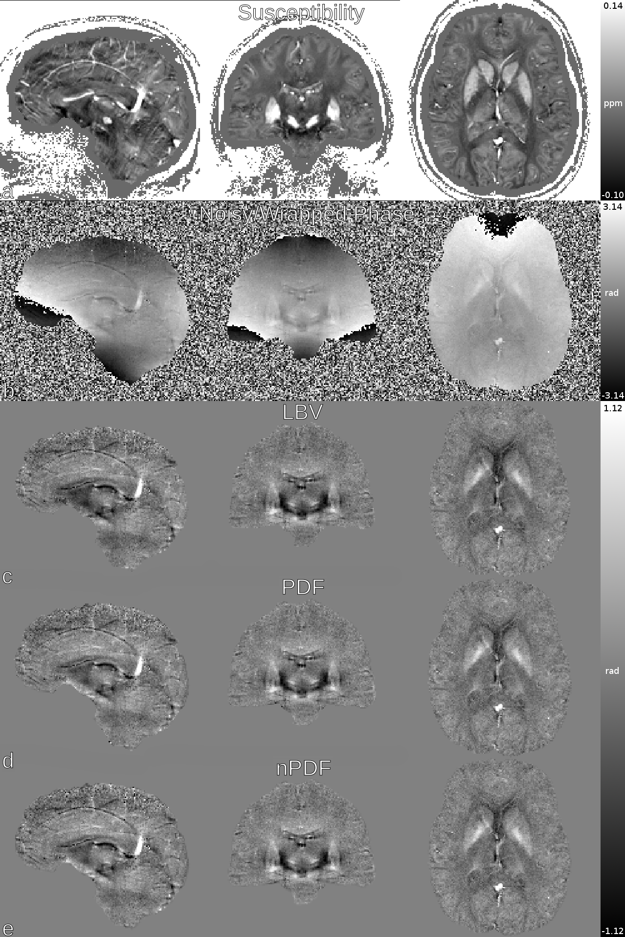
A) COSMOS7,8 ground-truth (3D spoiled-GRE on a 3T Siemens Tim Trio with 1.06-mm isotropic voxels, 240×196×120, TE/TR=25/35ms, 12 head orientations), from which a noisy field map was forward simulated with a widespread distribution of external sources. Background filtering was performed with LBV3, PDF9 and nonlinear-PDF adding a buffer region to reduce boundary errors (Fig. 1). Reconstructions were evaluated with RMSE, HFEN and SSIM metrics8.
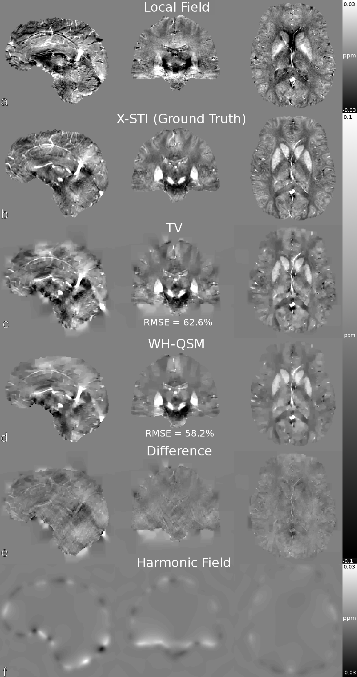
B) In vivo data (single 3T acquisition from protocol described above), where resulting reconstructions were evaluated with a previously proposed susceptibility-tensor derived ground-truth8,9.
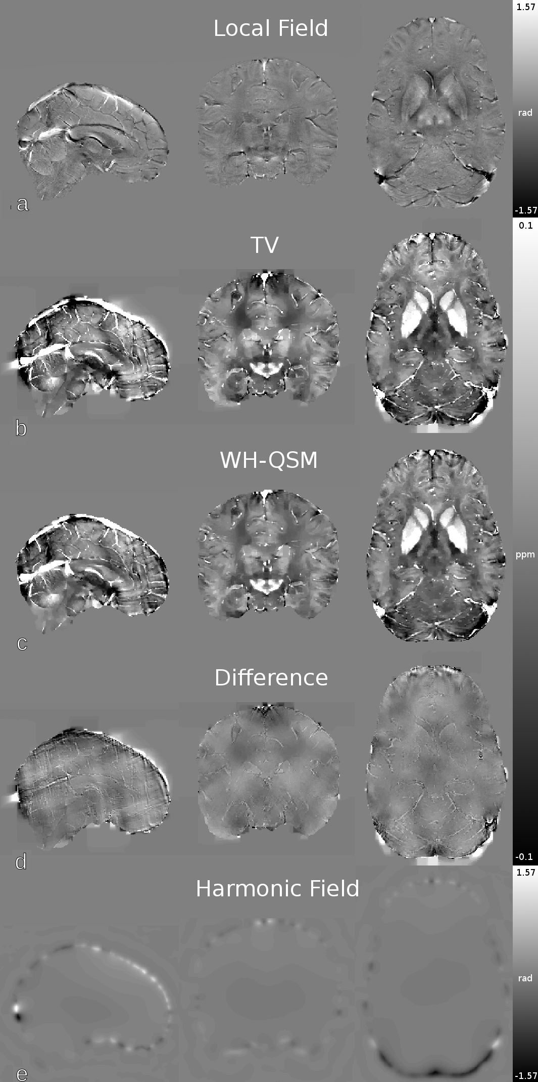
C) In vivo data (3T Siemens Trio with a 32-channel head coil, 0.8-mm isotropic voxels, 224×280×320, Temin/ΔTE/TR/TA=2.34ms/2.30ms/25ms/7:08min) processed with an in-house temporal unwrapping algorithm and subsequent magnitude-weighted nonlinear multi-echo combination.
In all experiments the regularization parameters were optimized for the reference (TV-only) method, and these were then propagated to the proposed method (WH-QSM) without further optimization.
Results
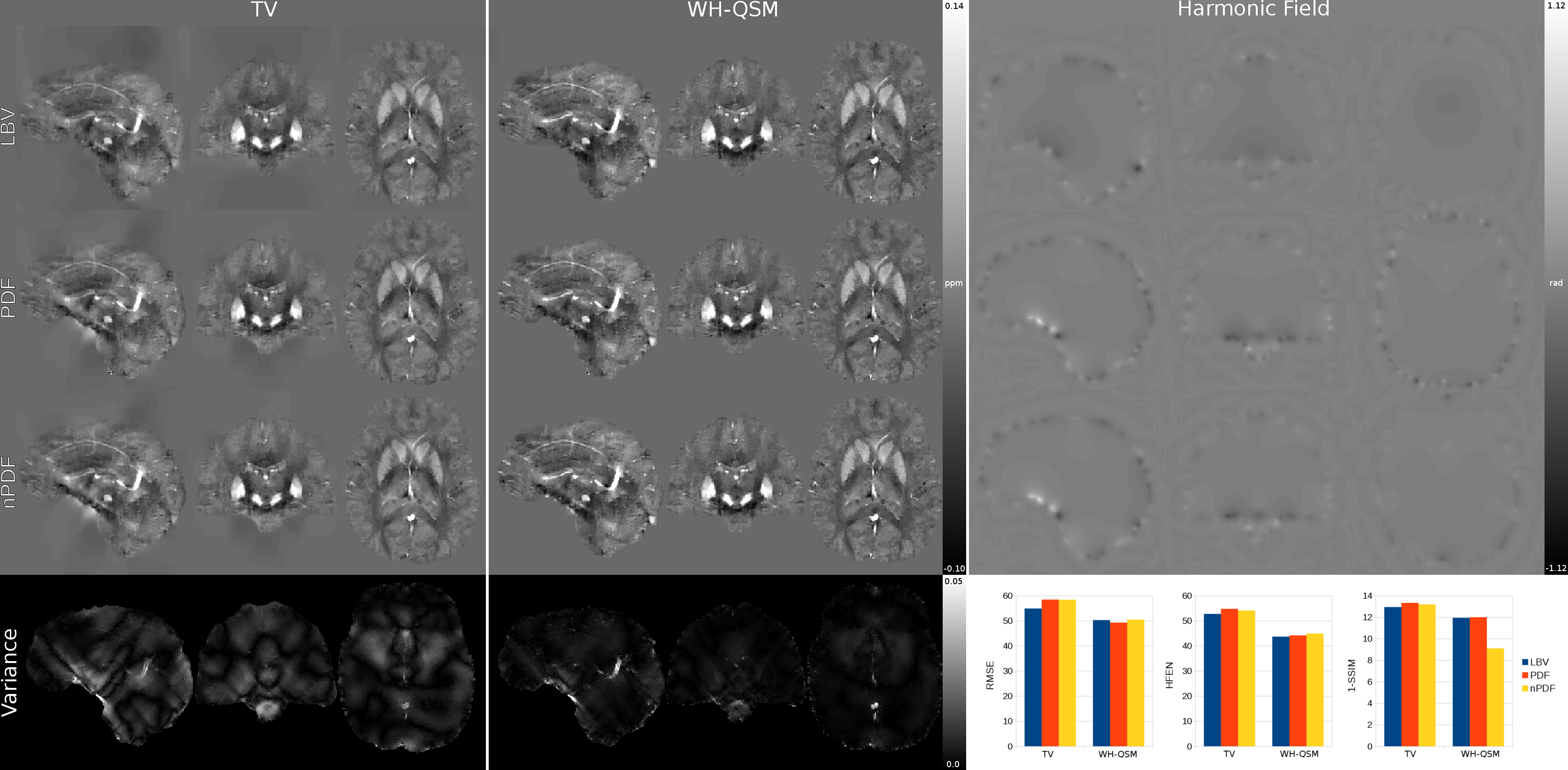
A) WH-QSM improved on the TV-QSM baseline behavior for all quality metrics and for all input data. On visual inspection, all WH-QSM reconstructions were qualitatively similar. Quantitatively, this was captured by lower global variance (Fig. 2).
B) WH-QSM returned a 4.4% improvement in RMSE with respect to TV-QSM when using Xsti as reference (Fig 3). A similar behavior was observed when using X33 as reference (77.3% RMSE for TV, 73.8% for WH-QSM), suggesting that the Challenge’s local phase data contained some background field remnants.
C) Qualitatively, WH-QSM reconstructions of sub-millimeter, multi-echo in vivo data returned less streaking artifacts than those for TV. This was particularly noticeable at the ROI boundary (Fig. 4).
Discussion & Conclusion
Our proposed algorithm consistently yielded results with less streaking artifacts and improved quality metrics. The WH-QSM algorithm was found to be robust with respect to input data variations; solutions were qualitatively similar regardless of the background pre-filtering method utilized – observation that was quantitatively confirmed by the variance maps. The new formulation incorporates two additional free parameters, though notably, outcome measures were relatively unaltered, i.e. remained close to optimal, for a wide range of parameter values, i.e. [100-1000] for beta and [10-100] for μh. These results indicate that WH-QSM may provide an additional robustness level to in-vivo data, with no significant processing penalty or complexity due to the introduction of new parameters.Acknowledgements
FONDECYT 1161448, CONICYT Programa PIA Anillo ACT1416, Becas de Doctorado Nacional CONICYT Folio 21150369 and Wellcome-UK [203147/Z/16/Z].
References
1. Li L, Leigh JS. Quantifying arbitrary magnetic susceptibility distributions with MR. Magn. Reson. Med. 2004; 51: 1077–1082.
2. Li L, Leigh JS. High-precision mapping of the magnetic field utilizing the harmonic function mean value property. J. Magn. Reson. 2001; 148: 442–448.
3. Zhou D, Liu T, Spincemaille P, Wang Y. Background field removal by solving the Laplacian boundary value problem. NMR in Biomedicine. 2014;27(3):312–319.
4. Bilgic B, Chatnuntawech I, Langkammer C, Setsompop K. Sparse Methods for Quantitative Susceptibility Mapping. Wavelets and Sparsity XVI, SPIE 2015. doi: 10.1117/12.2188535
5. Zhao B, Setsompop K, Ye H, Cauley S. and Wald LL. Maximum likelihood reconstruction for magnetic resonance fingerprinting, IEEE Trans Med Imaging 2016;35:1812-1823.
6. Milovic C, Bilgic B, Zhao B, Acosta-Cabronero J, Tejos C. A Fast Algorithm for Nonlinear QSM Reconstruction with Variational Penalties. Proceedings of the Fourth International Workshop on MRI Phase Contrast & Quantitative Susceptibility Mapping. 2016;1:132.
7. Liu T, Spincemaille P, De Rochefort L, Kressler B, Wang Y. Calculation of susceptibility through multiple orientation sampling (COSMOS): A method for conditioning the inverse problem from measured magnetic field map to susceptibility source image in MRI. Magnetic Resonance in Medicine. 2009;61(1):196–204.
8. Langkammer C, Schweser F, Shmueli K, Kames C, Li X, Guo L, Milovic C, Kim J, Wei H, Bredies K, Buch K, Guo Y, Liu Z, Meineke J, Rauscher A, Marques JP and Bilgic B. Quantitative Susceptibility Mapping: Report from the 2016 Reconstruction Challenge. Magn. Reson. Med. doi:10.1002/mrm.26830
9. Milovic C, Bilgic B, Langkammer C, Acosta-Cabronero J, Tejos C. Quantitative Susceptibility Mapping (QSM) challenge follow-up: analysis of susceptibility ground-truth and quality metrics. Proceedings of the ESMRMB 2017, Barcelona.
Figures