2201
Fast and accurate reconstruction for susceptibility source separation in QSM1Department of Statistics, Seoul National University, Seoul, Republic of Korea, 2Laboratory for Imaging Science and Technology, Department of Electrical and Computer Engineering, Seoul National University, Seoul, Republic of Korea
Synopsis
We investigate fast and accurate reconstruction methods for susceptibility source separation (S3) in quantitative susceptibility mapping (QSM). S3 separates positive and negative susceptibility sources within a voxel utilizing signal relaxation (R2') for dipole inversion. We propose new primal-dual (PD) methods for S3 and compare them with the alternating Gauss-Newton conjugate gradient (A-GNCG). A-GNCG alters the energy functional, and furthermore its convergence is not guaranteed. In contrast, the proposed PD methods are exact and have convergence guarantees. Validation on a simulated phantom and in-vivo data shows that the PD methods converge faster with better accuracies.
Purpose
Susceptibility source separation (S3)1 is a method that separates positive and negative parts in QSM to distinguish positive (e.g., iron) and negative (e.g., myelin) susceptibility sources (relative to water) within the same voxel. We propose primal-dual (PD) methods for this problem. Our PD methods are significantly faster and more accurate than the alternating Gauss-Newton conjugate gradient (A-GNCG) method previously employed for S31. Moreover, A-GNCG may not converge or results in a suboptimal reconstruction.Theory
1) S3 Problem
S3 is posed as a variant of morphology-enabled dipole inversion (MEDI)2, which minimizes the energy functional$$\frac{1}{2}\left(\|W_p(b_p-D_p(\chi_{pos}-\chi_{neg})\|_2^2+\|W_m(b_m-D_m(\chi_{pos}+\chi_{neg})\|_2^2 \right)+\lambda(\|MG\chi_{pos}\|_1+\|MG\chi_{neg}\|_1),$$where $$$\chi_{pos}\ge{0}$$$ and $$$\chi_{neg}\ge{0}$$$ are the positive and negative parts of the susceptibility map; $$$b_m$$$ is frequency shift from magnetic perturbation; $$$b_p$$$ is the magnitude signal relaxation ($$$R_2'=R_2^*-R_2$$$); $$$D_p$$$ and $$$D_m$$$ are matrices induced by the dipole and magnitude decay kernels, respectively. SNR-weighting diagonal matrices for phase and magnitude are respectively denoted by $$$W_p$$$ and $$$W_m$$$. $$$M$$$ is the edge indicator map derived from the magnitude image, and $$$G$$$ is the gradient operator. The third and fourth terms are nonsmooth regularization terms to reduce streaking artifacts. Unlike the classical MEDI, this is a constrained optimization problem.
2) A-GNCG
In the A-GNCG1the $$$L_1$$$-norm $$$\|x\|_1=\sum_{i=1}^n|x_i|$$$ is smoothly approximated by $$$\sum_{i=1}^n\sqrt{x_i^2+\epsilon}$$$. Then the energy functional becomes differentiable and the resulting Euler-Lagrangian equation is$$(W_pD_p)^*(W_pD_p(\chi_s-\chi_{s'})-b_p))+(W_mD_m)^*(W_mD_m(\chi_s+\chi_{s'})-b_m))+\lambda(MG)^*\mathcal{S}(MG\chi_s)=0,$$where $$$s=pos$$$ and $$$s'=neg$$$ or vice versa, and$$\mathcal{S}(x)=(x_1/\sqrt{x_1^2+\epsilon},\dotsc,x_n/\sqrt{x_n^2+\epsilon}),$$is solved by alternatingly updating $$$\chi_{pos}$$$ and $$$\chi_{neg}$$$ using GNCG. For each inner iteration, the updated components are projected onto the nonnegative orthant to meet the constraints. Not only this smoothing alters the energy functional, but also convergence of this algorithm is not guaranteed. Moreover, there is no guideline for choosing the smoothing parameter $$$\epsilon$$$.
3) PD
The PD methods are based on the variational formulation of the $$$L_1$$$-norm: $$$\lambda\|x\|_1=\max_{\|y\|_\infty\le\lambda}x^*y$$$. To solve the resulting saddle-point problem, we propose to employ the Condat-Vũ algorithm (PD-CV)3-4$$w_m^k=D_m^*(W_m^*W_m)D_m(\chi_{pos}^k+\chi_{neg}^k)-D_m^*W_m^*b_m\\w_p^k=D_p^*(W_p^*W_p)D_p(\chi_{pos}^k-\chi_{neg}^k)-D_p^*W_p^*b_p\\\chi_{pos}^{k+1}=P_{[0,\infty)}(\chi_{pos}^k-\tau(w_m^k+w_p^k+(MG)^*y_{pos}^k))\\\chi_{neg}^{k+1}=P_{[0,\infty)}(\chi_{neg}^k-\tau(w_m^k-w_p^k+(MG)^*y_{neg}^k))\\\tilde{\chi}_{pos}^{k+1}=2\chi_{pos}^{k+1}-\chi_{pos}^k\\\tilde{\chi}_{neg}^{k+1}=2\chi_{neg}^{k+1}-\chi_{neg}^k\\y_{pos}^{k+1}=P_{[-\lambda,\lambda]}(y_{pos}^k+\sigma{MG}\tilde{\chi}_{pos}^{k+1})\\y_{neg}^{k+1}=P_{[-\lambda,\lambda]}(y_{neg}^k+\sigma{MG}\tilde{\chi}_{neg}^{k+1})$$and the Loris-Verhoeven algorithm (PD-LV)5-6$$w_m^k=D_m^*(W_m^*W_m)D_m(\chi_{pos}^k+\chi_{neg}^k)-D_m^*W_m^*b_m\\w_p^k=D_p^*(W_p^*W_p)D_p(\chi_{pos}^k-\chi_{neg}^k)-D_p^*W_p^*b_p\\\tilde{\chi}_{pos}^{k+1}=P_{[0,\infty)}(\chi_{pos}^k-\tau(w_m^k+w_p^k+(MG)^*y_{pos}^k))\\\tilde{\chi}_{neg}^{k+1}=P_{[0,\infty)}(\chi_{neg}^k-\tau(w_m^k-w_p^k+(MG)^*y_{neg}^k))\\y_{pos}^{k+1}=P_{[-\lambda,\lambda]}(y_{pos}^k+\sigma{MG}\tilde{\chi}_{pos}^{k+1})\\y_{neg}^{k+1}=P_{[-\lambda,\lambda]}(y_{neg}^k+\sigma{MG}\tilde{\chi}_{neg}^{k+1})\\\chi_{pos}^{k+1}=P_{[0,\infty)}(\chi_{pos}^k-\tau(w_m^k+w_p^k+(MG)^*y_{pos}^{k+1}))\\\chi_{neg}^{k+1}=P_{[0,\infty)}(\chi_{neg}^k-\tau(w_m^k-w_p^k+(MG)^*y_{neg}^{k+1})),$$where $$$P_I(x)$$$ denotes the coordinatewise projection of $$$x$$$ onto interval $$$I$$$. Note $$$W_m^*W_m$$$ and $$$W_p^*W_p$$$ are trivial to compute. Both algorithms enjoy guaranteed convergence with a proper choice of step size parameters $$$(\sigma,\tau)$$$3-6.
Methods
SIMULATION: a geometric phantom was developed to validate the proposed methods. Seven different cylinders were contained in one large cylinder with different compositions of susceptibility values. $$$R_2$$$ was set to 10Hz for all positions; $$$R_2'$$$ and frequency shift maps were generated based on the susceptibility model.
IN-VIVO EXPERIMENTS: five healthy volunteers (age=25.6±3.2 years) were scanned at 3T MRI (Siemens Tim Trio, Erlangen, Germany) using a 32-channel phased-array head coil. All volunteers signed a written consent form approved by the institutional review board. After three plane localization and $$$B_0$$$ shimming, three scans were acquired to estimate $$$R_2^*$$$ (and frequency shift) and $$$R_2$$$. To estimate $$$R_2^*$$$ and frequency shift, 3D multi-echo GRE data were acquired with the following parameters: FOV=192×192×96mm3, voxel size=1×1×2mm3, TR=64ms, TE=2.9-25.9ms with echo spacing=4.6ms, navigation echo TE=36.0ms, flip angle=22°, and total acquisition time=7:02 min. For $$$R_2$$$ estimation, 2D multi-echo SE data were acquired with the following parameters: FOV=192×192mm2, voxel size=1×1mm2, slice thickness=2mm, number of slices=36, TR=4800ms, TE=20-120ms with echo spacing of 20ms, flip angle=90°, and acquisition time=7:09min. Frequency shift and $$$R_2'$$$ estimations were the same as the literature1.
Results
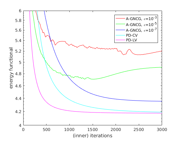
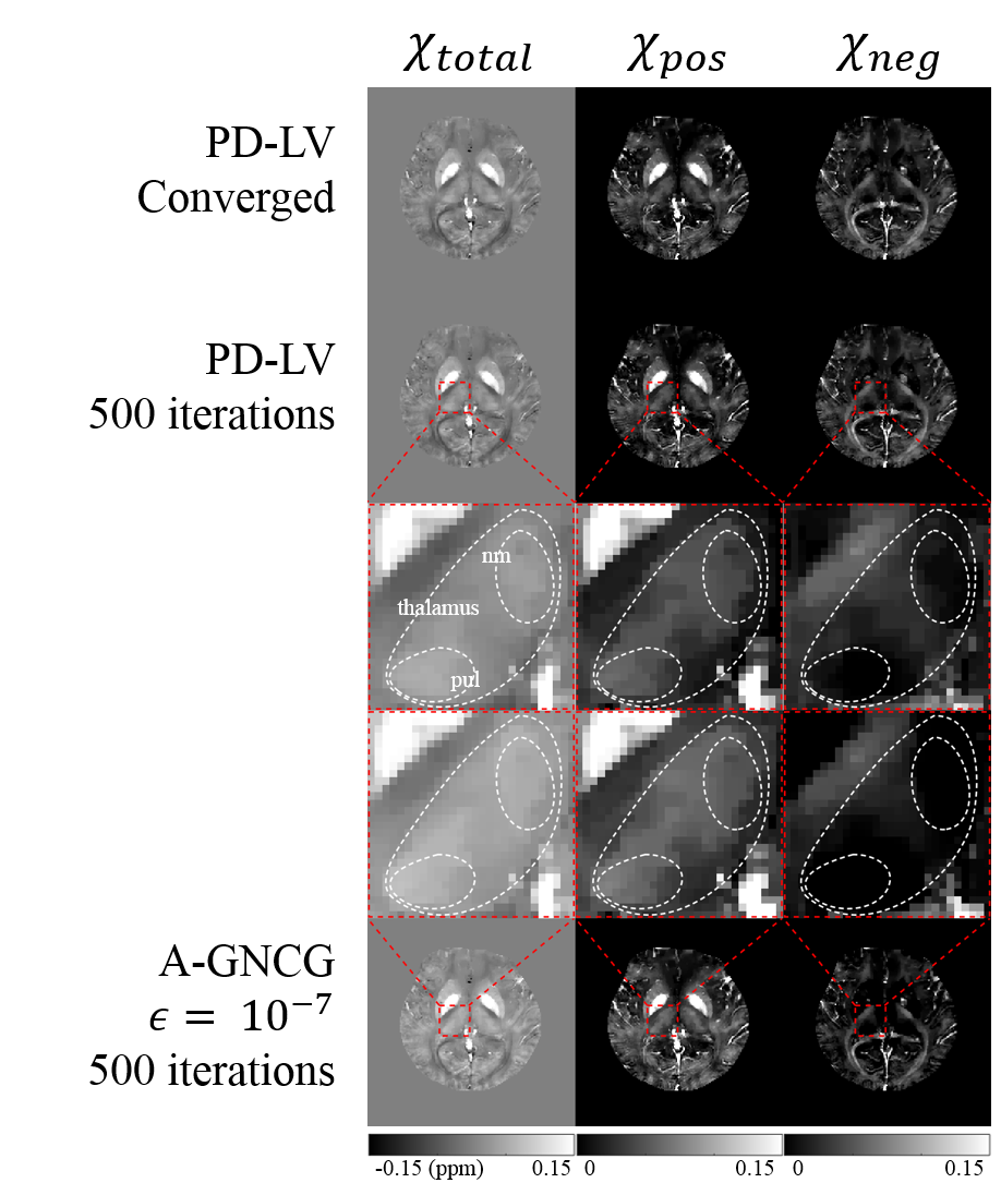
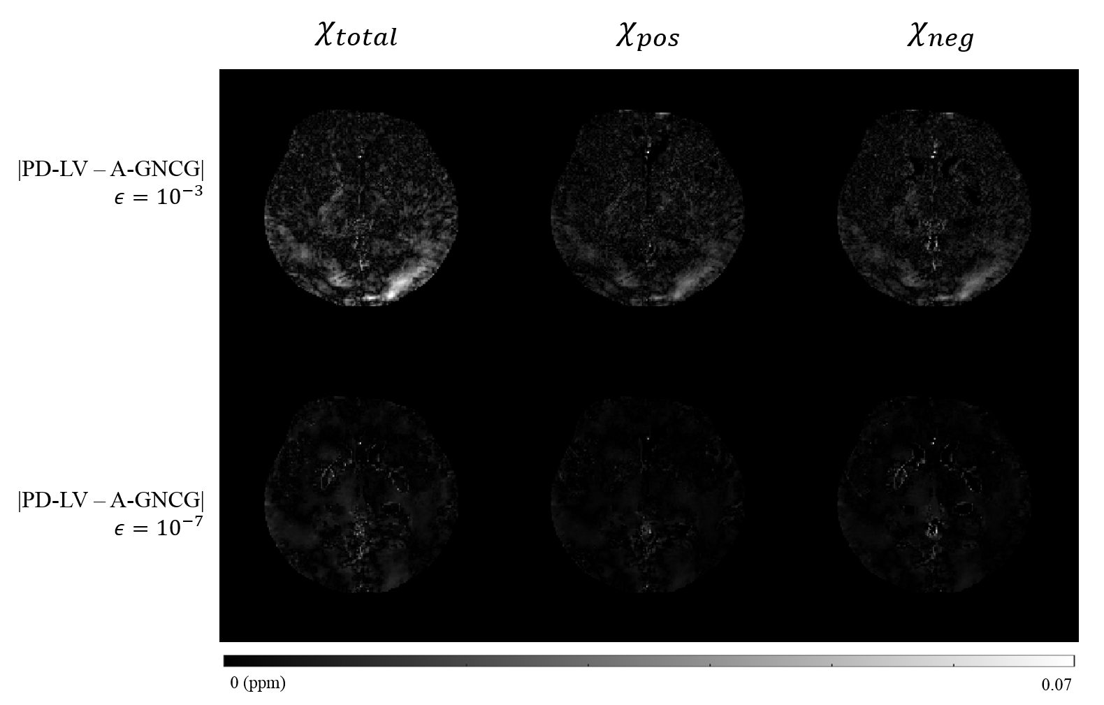
Convergence behavior of the methods on the geometric phantom and the in-vivo data is shown in Figs. 1-2, respectively. Figs. 3-4 compare the reconstructions obtained by A-GNCG and PD methods. Fig. 5 presents correlation between known iron concentration7-8 and susceptibility map obtained from the employed methods.Discussion
Overall, PD-LV was the fastest (Figs. 1-2) and exhibited better accuracy even when terminated early (Figs. 3-5). Accuracy of A-GNCG highly depends on the value of $$$\epsilon$$$. For a large $$$\epsilon$$$, it deviates significantly form the original problem and may not converge at all. A small $$$\epsilon$$$ approximates the original problem better, but the numerical conditioning of the Euler-Lagrange equation becomes poorer, and may reach an inaccurate, suboptimal solution. In contrast, PD-LV and PD-CV solve the exact non-smooth optimization problem directly, and reach a sufficiently optimal solution within 500-1000 iterations, enabling fast and accurate reconstruction. Since both PD algorithms consist only of matrix-vector multiplication and coordinatewise projections, the reconstruction time can be reduced up to 10 times using GPUs. In addition, PD-LV allows more flexible parameter selection5-6, contributing to its faster convergence.
The Chambolle-Pock (CP) algorithm9 was employed for a PD formulation of the classical MEDI10. When applied to S3, CP results in a more complex update rule than PD-LV or PD-CV due to the constrained nature of the problem. Even when applied to the classical MEDI, PD-LV and PD-CV yield simpler rules.
Acknowledgements
This work was supported by the National Research Foundation of Korea (NRF) grants funded by the Korea government (MSIP) (No. 2014R1A4A1007895).References
1. Lee J, Nam Y, Choi JY, Shin H, Hwang T, Lee J. Separating positive and negative susceptibility sources in QSM. In ISMRM 2017.
2. Liu J, Liu T, de Rochefort L, Dedoux J, Khalidov I, Chen W, Tsiouris AJ, Wisnieff C, Spincemaille P, Prince MR, Wang Y. Morphology enabled dipole enversion for quantitive susceptibility mapping using structural consistency between the magnitude image and the susceptibility map. Neuroimage 59.3 (2012):2560-2568.
3. Condat L. A primal-daul splitting method for convex optimization involving Lipschitzian, prooximable and linear composite terms. Journal of Optimization Theory and Applications 158.2 (2013):460-479.
4. Vũ BC. A splitting algorithm for dual monotone inclusions involving cocoercive operators. Advances in Computational Mathematics 38.3 (2013): 667-681.
5. Loris I, and Verhoeven C. On a generalization of the iterative soft-thresholding algorithm for the case of non-separable penalty. Inverse Problems 27.12 (2011): 125007.
6. Chen P, Huang J, and Zhang X. A primal-dual fixed point algorithm for minimization of the sum of three convex separable functions. Fixed Point Theory and Applications 2016.1 (2016): 54.
7. Schweser F, Deistung A, Lehr BW, Reichenbach JR. Quantitative imaging of intrinsic magnetic tissue properties using MRI signal phase: an approach to in vivo brain iron metabolism? Neuroimage 54.4 (2011): 2789-2807.
8. Langkammer C, Schweser F, Krebs N, et al. Quantitative susceptibility mapping (QSM) as a means to measure brain iron? A post mortem validation study. Neuroimage 62.3 (2012): 1593-1599.
9. Chambolle A, and Pock T. A first-order primal-dual algorithm for convex problems with applications to imaging. Journal of mathematical imaging and vision 40.1 (2011): 120-145.
10. Kee Y, et al. Primal‐dual and forward gradient implementation for quantitative susceptibility mapping. Magnetic Resonance in Medicine (2017). In Press.
Figures
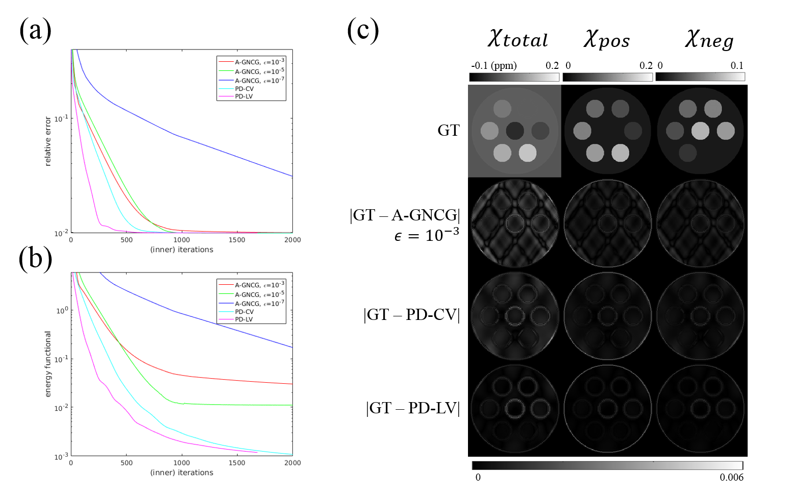
(a) Relative error vs iteration for the simulation study. PD-LV was the fastest to achieve the lowest relative error.
(b) Energy functional value vs iteration. All the A-GNCG instances converged to suboptimal points. Time to achieve the level of PD-LV at 500th iteration was 89.1s/92.3s/>300s for PD-LV/PD-CV/A-GNCG (all $$$\epsilon$$$s). Time per iteration was 0.18s/0.14s/0.12s/0.11s/0.11s for PD-LV/PD-CV/A-GNCG $$$\epsilon=10^{-3}$$$/$$$10^{-5}$$$/$$$10^{-7}$$$. Without GPU acceleration, it was 2.58s/2.54s/1.33s/1.33s/1.33s.
(c) Ground truth susceptibility maps and its difference from reconstructions with A-GNCG ($$$\epsilon=10^{-3}$$$), PD-CV and PD-LV terminated after 500 iterations. A-GNCG with smaller $$$\epsilon$$$s exhibited larger errors due to premature convergence.
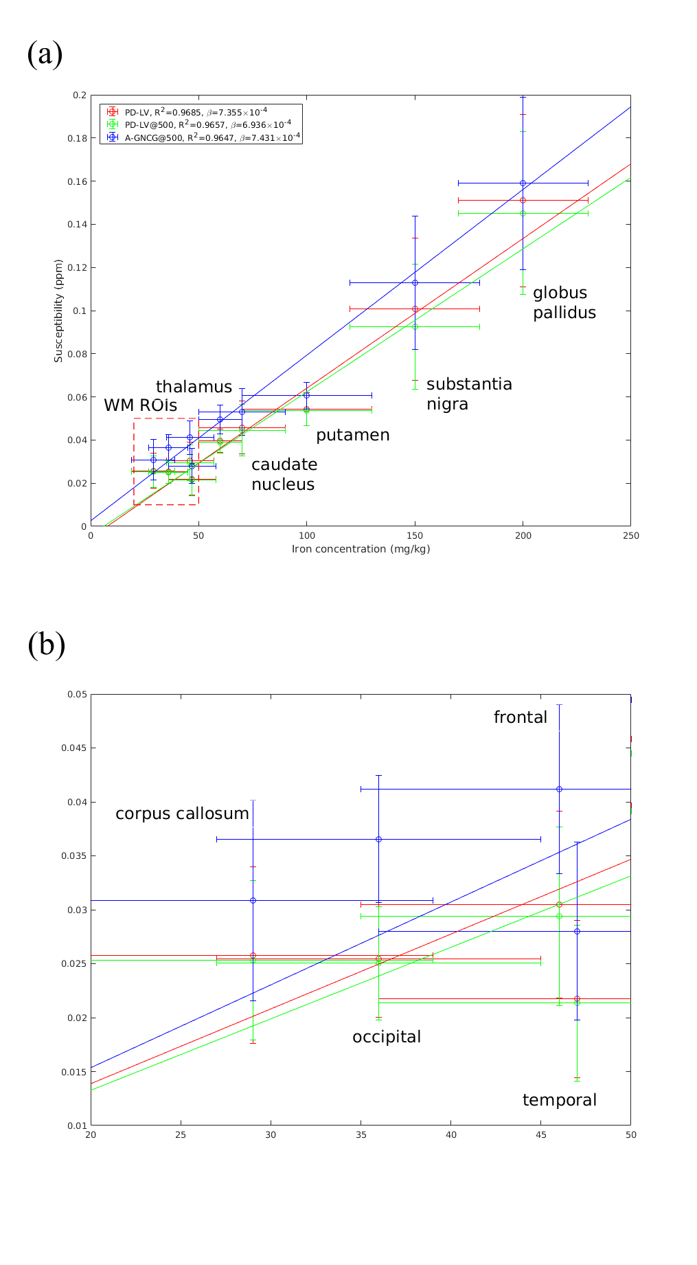
(a) Estimated positive susceptibility ($$$\chi_{pos}$$$) from converged PD-LV, early-stopped PD-LV and A-GNCG $$$\epsilon=10^{-7}$$$ at 500 interations, with respect to literature values of iron concentration ROIs. Converged PD-LV shows a strong ($$$R^2=.9685$$$) linear relationship with iron concentration, a dominant positive susceptibility source. Early-stopped PD-LV ($$$R^2=.9657$$$) exhibits a reduced but slightly better than A-GNCG ($$$R^2=.9647$$$) correlation. Furthermore, the estimated slope of the early-stopped PD-LV ($$$6.60\pm0.27\times{10^{-4}}$$$) is closer to the converged value ($$$6.91\pm0.28\times{10^{-4}}$$$) than A-GNCG ($$$7.65\pm0.28\times 10^{-4}$$$).
(b) White matter (WM) ROIs portion enlarged.