Synopsis

In this work, we explored an alternative approach of using nominal $$$R_2^{\:'}$$$ instead of measured $$$R_2^{\:'}$$$ in separating the two susceptibility sources. The linear relationship between $$$R_2^{*}$$$ and $$$R_2^{\:'}$$$ was investigated and used to obtain the nominal $$$R_2^{\:'}$$$ values. The positive and negative magnetic susceptibility source maps using nominal $$$R_2^{\:'}$$$ showed similar susceptibility distribution to the map using measured $$$R_2^{\:'}$$$.

Introduction

Recently, a new QSM algorithm that separates positive and negative susceptibility sources was proposed [1]. The method requires the estimation of $$$R_{2}^{\:'}$$$ which is defined as $$$R_{2}^{*}-R_{2}$$$ and, therefore, needs $$$R_{2}$$$ measurement. However, acquiring $$$R_{2}$$$ requires long scan time (10 min) and processing time (up to several hours) [2] and is not commonly performed in neuroimaging. In this work, we explored an alternative approach of using nominal $$$R_{2}^{\:'}$$$ instead of measured $$$R_{2}^{\:'}$$$ (= $$$R_{2,measured}^{\:'}$$$) in susceptibility source separation. The method was applied to healthy volunteers and multiple sclerosis (MS) patients and the resulting susceptibility maps were compared with those from $$$R_{2,measured}^{\:'}$$$.

Methods

[Estimating Nominal $$$R_{2}^{\:'}$$$]

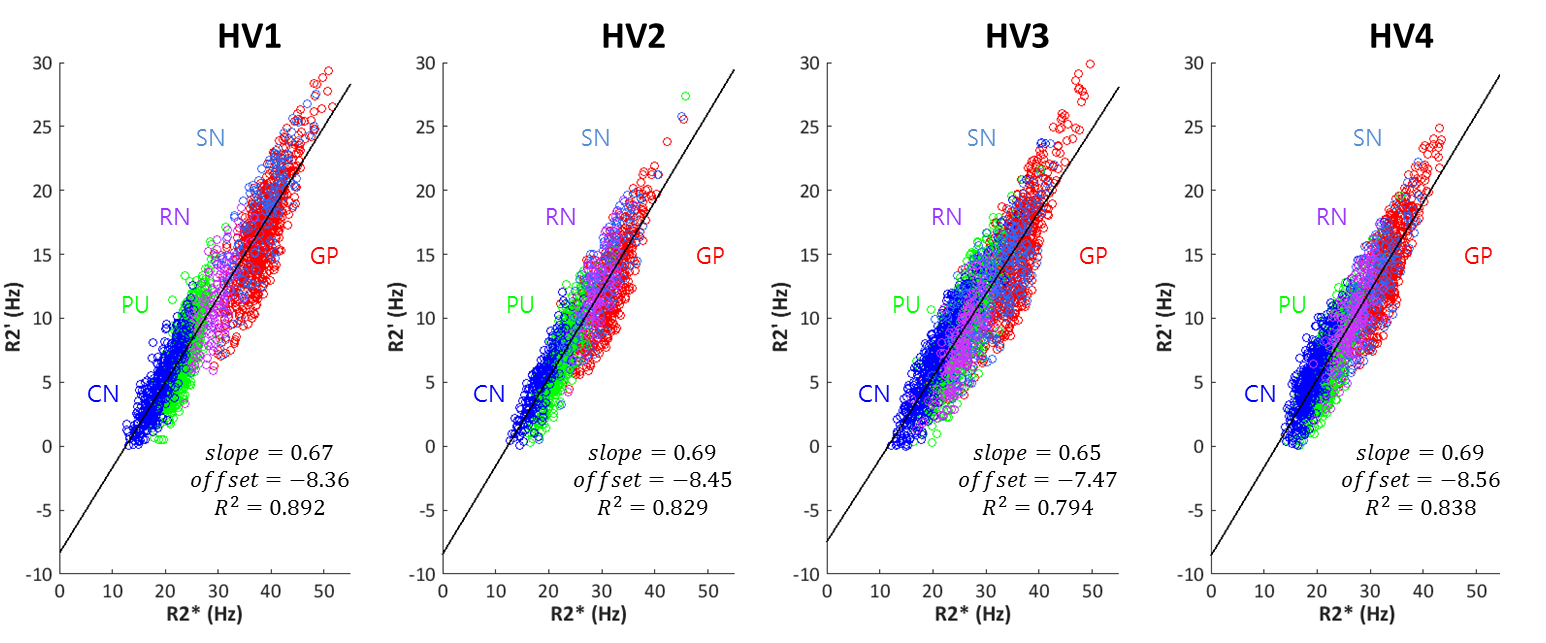
It has been shown that both $$$R_{2}^{\:'}$$$ and $$$R_{2}^{*}$$$ can be modeled as a linear equation to tissue susceptibility concentration [3-5]. Therefore, we can infer that the relationship between $$$R_{2}^{\:'}$$$ and $$$R_{2}^{*}$$$ is also linear. It can be written as follows:$$R_{2}^{\:'} = a\cdot{R_{2}}^{*}+b\:\:\:\:\:\:Eq. [1]$$ Once the two coefficients, $$$a$$$ and $$$b$$$, are known, we can use $$$R_{2}^{*}$$$ to estimate a nominal value of $$$R_{2}^{\:'}$$$. To obtain the coefficients, two different approaches are tested. First, the measurements in a literature [3] lead to $$$a=0.78$$$ and $$$b=-6.07$$$. The estimated $$$R_{2}^{\:'}$$$ using these values is referred to as $$$R_{2,nominal,lit.}^{\:'}$$$ hereafter. The second approach is to acquire $$$R_{2}^{*}$$$ and $$$R_{2,measured}^{\:'}$$$ from in-vivo data and then generate the coefficients using linear regression. This $$$R_{2}^{\:'}$$$ is referred to as $$$R_{2,nominal,fit}^{\:'}$$$.

[Experiments and data processing]

Four healthy volunteers and three MS patients were scanned at 3T. For $$$R_{2}^{*}$$$, gradient-echo was acquired (healthy volunteers: resolution=1×1×2mm³, TR=53ms, and TE=5.1:5.0:30.0ms; MS patients: resolution=0.5×0.5×2mm³, TR=53ms, and TE=5.8:6.2:36.7ms). To estimate $$$R_{2,measured}^{\:'}$$$, $$$R_{2}$$$ was acquired using multi-echo spin-echo (healthy volunteers: resolution=1×1×2mm³, TR=2400ms, and TE=10:10:100ms; MS patients: resolution=0.5×0.5×2mm³, TR=1800ms, and TE=10:10:90ms). An $$$R_{2}^{*}$$$ map was generated by mono-exponential fitting to the multi-echo data. An $$$R_{2}$$$ map was generated after $$$EPG_{SLR}$$$ correction [2]. $$$R_{2}^{\:'}$$$ was calculated by subtracting $$$R_{2}$$$ from $$$R_{2}^{*}$$$. The positive and negative susceptibility maps were acquired using [1].

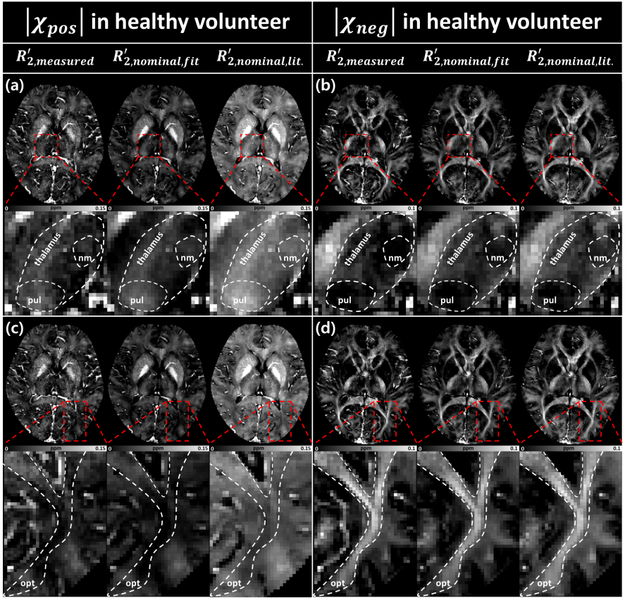
To estimate the coefficients of $$$R_{2,nominal,fit}^{\:'}$$$, a linear regression between $$$R_{2}^{*}$$$ and $$$R_{2,measured}^{\:'}$$$ was performed for voxels in five regions (SN, RN, CN, GP and PU) in healthy volunteers. No white matter region was included as $$$R_{2}^{*}$$$ has been shown to depend on not only susceptibility concentration but also fiber orientation [6, 7]. Outliers were removed using Cook’s distance [8]. The positive and negative susceptibility source maps from $$$R_{2,measured}^{\:'}$$$, $$$R_{2,nominal,fit}^{\:'}$$$, and $$$R_{2,nominal,lit.}^{\:'}$$$ were generated and compared. Thalamus, which includes iron-rich but myelin-lacking nuclei (pulvinar and nucleus medialis), and optic-radiation, which has myelin-rich but iron lacking region, were inspected [9-11]. The results were also compared in MS lesions.

Results

When relationship between $$$R_{2}^{*}$$$ and $$$R_{2}^{\:'}$$$ was explored, it showed a good linear relation (Fig. 1), agreeing with previous studies [3-5]. The slopes and offsets in [Eq. 1] of four healthy volunteers have similar values with small standard deviation ($$$slope=0.675\pm0.021$$$ and $$$offset=-8.21\pm0.499$$$). Hence, we used $$$R_{2,nominal,fit}^{\:'}=0.675\cdot{R_{2}}^{*}-8.21$$$ hereafter. From the literature [3], we found $$$R_{2,nominal,lit.}^{\:'}=0.78\cdot{R_{2}}^{*}-6.07$$$. The positive and negative susceptibility source maps of a healthy volunteer are shown in Fig. 2. Overall, the maps show similar contrast distribution. However, the positive susceptiblity map using $$$R_{2,nominal,lit.}^{\:'}$$$ was slightly overestimated (Fig. 2a and c right column). When thalamus was zoomed in, pulvinar and nucleus medialis are delineated in the negative susceptibility maps using $$$R_{2,measured}^{\:'}$$$ and $$$R_{2,nominal,fit}^{\:'}$$$ images (Fig. 2a and b left column and middle column).

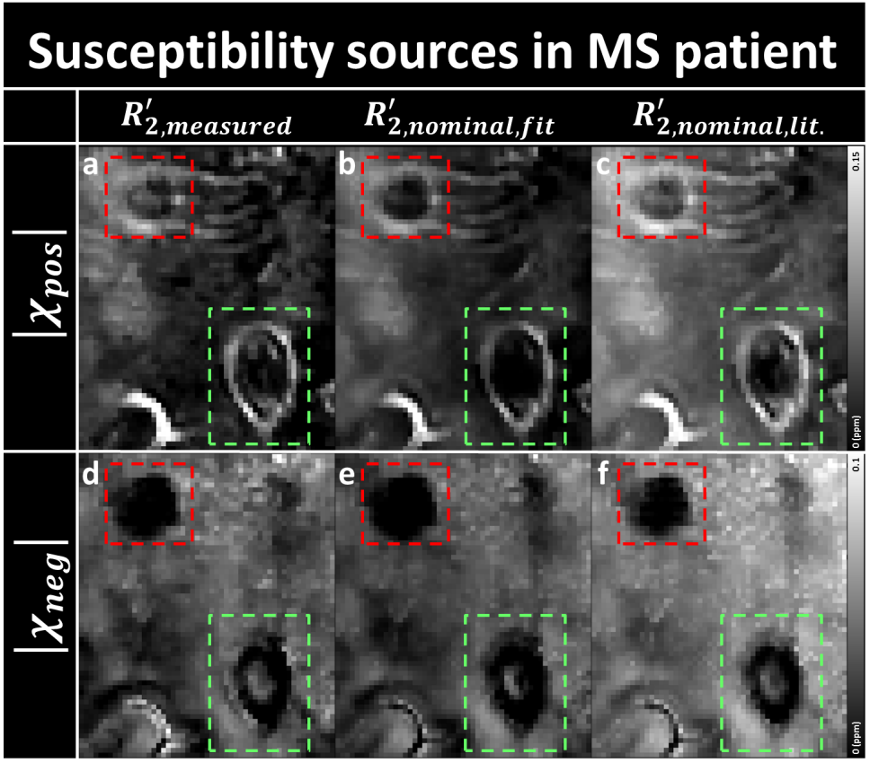
In MS patient results, all the positive maps show two ring-shaped lesions (Fig. 3), indicating iron accumulation at the rim of the lesions [12]. One of them shows potentially a feeding vein inside the lesion (Fig. 3; red box), which was still detectable but less apparent in the nominal $$$R_{2}^{\:'}$$$ corrected images. The negative map using $$$R_{2,measured}^{\:'}$$$ shows a demyelinated lesion (Fig. 3d and e; green box), and a potentially partially remyelinated lesion (Fig. 3d and e; red box). Similar appearances are observed in the negative susceptibility maps using $$$R_{2,nominal,fit}^{\:'}$$$, and $$$R_{2,nominal,lit.}^{\:'}$$$.

Discussion and Conclusion

Acknowledgements

References

[1] Lee, Jingu et al. “Separating positive and negative susceptibility sources in QSM.” ISMRM conference (2017).

[2] McPhee KC, Wilman AH. Transverse relaxation and flip angle mapping: Evaluation of simultaneous and independent methods using multiple spin echoes. Magn Reson Med 2017;77(5):2057-2065.

[3] Sedlacik, Jan, et al. "Reversible, irreversible and effective transverse relaxation rates in normal aging brain at 3T." Neuroimage 84 (2014): 1032-1041.

[4] C Langkammer, et al. “Quantitative MR imaging of brain iron: a postmortem validation study“, Radiology 257 (2010)

[5] Yao, Bing, et al. "Susceptibility contrast in high field MRI of human brain as a function of tissue iron content." Neuroimage 44.4 (2009): 1259-1266.

[6] Lee, Jongho, et al. "Sensitivity of MRI resonance frequency to the orientation of brain tissue microstructure." Proceedings of the National Academy of Sciences 107.11 (2010): 5130-5135.

[7] Lee, Jingu, et al. "An R2* model of white matter for fiber orientation and myelin concentration." NeuroImage 162 (2017): 269-275.

[8] Cook, R. Dennis. "Detection of influential observation in linear regression." Technometrics 19.1 (1977): 15-18.

[9] Duyn, Jeff H., and John Schenck. "Contributions to magnetic susceptibility of brain tissue." NMR in biomedicine 30.4 (2017).

[10] Bender, B., et al. Optimized 3D magnetization-prepared rapid acquisition of gradient echo: identification of thalamus substructures at 3T. American Journal of Neuroradiology 32.11 (2011): 2110-2115.

[11] Drayer, Burton, et al. Magnetic resonance imaging of brain iron. American journal of neuroradiology 7.3 (1986): 373-380.

[12] Zhang, Y., et al. "Quantitative susceptibility mapping and R2* measured changes during white matter lesion development in multiple sclerosis: myelin breakdown, myelin debris degradation and removal, and iron accumulation." American Journal of Neuroradiology 37.9 (2016): 1629-1635.