Synopsis

In this study, we proposed a novel QSM image reconstruction algorithm using annihilating filter‑based low-rank hankel matrix (ALOHA) approach. Unlike the conventional algorithm that requires additional anatomical information, the proposed method estimates susceptibility map using direct 3-D k-space domain interpolation in the Fourier domain. The proposed method showed superior performance over the conventional methods (SWIM, TSVD, TKD, MEDI, and TVSB) in a numerical phantom and in-vivo human brains.

Introduction

Methods

Theory

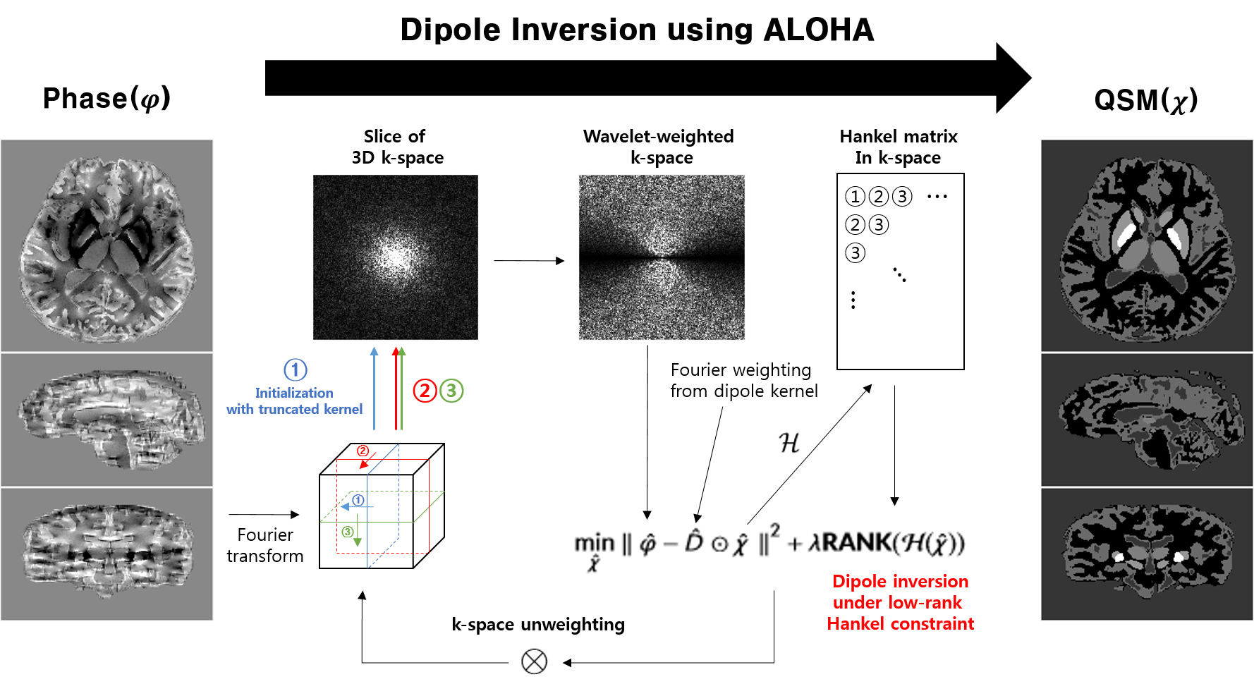
As demonstrated in the algorithm called ALOHA⁵, the redundancy in the spatial domain results in the low-rank Hankel structured matrix in Fourier domain. This implies that an artifact-free k-space data can be recovered from incomplete or distorted k-space measurement data by constructing Hankel structured matrix and exploiting its low-rankness⁵. Accordingly, we adopted this idea to solve the QSM dipole inversion problem. Specifically, the artifact-free k-space data estimation problem can be formulated as follows:

$$\min_{\hat{\chi}}{\parallel\hat{\varphi}-\hat{D}\odot\hat{\chi}\parallel}^2+\lambda{\bf RANK}(\mathcal{H(\hat{\chi})})$$

where $$$\hat{\varphi}$$$ denotes the Fourier data from a phase image, $$$\hat{D}$$$ is the spectrum of the dipole kernel, $$$\hat{\chi}$$$ is the Haar wavelet spectrum-weighted k-space image for enhancing data sparsity, $$$\odot$$$ is the Hadammard product, $$$\lambda$$$ is the regularization parameter, and $$$\mathcal{H(\cdot)}$$$ is the operator for Hankel transform. Since direct rank minimization is not possible, the following form of minimization is widely used.

$$\min_{U,V:\mathcal{H}(\hat{\chi})=UV^H}{\frac{1}{2}{\parallel \hat{\varphi}-\hat{D}\odot\hat{\chi}\parallel}^2+\frac{\lambda}{2}({\parallel{U}\parallel}_F^2+{\parallel{V}\parallel}_F^2)}\cdots(1)$$

The problem can be then solved using alternating direction method of multipliers (ADMM) algorithm. To reduce the computational burden and to avoid huge 3-D Hankel structured matrix, we address the optimization problem as a successive 2-D k-space interpolation problem along each axis. Specifically, to generate QSM maps that are not dependent on the processing direction, we first applied it along one direction of the 3-D k-space first, and then sequentially applied it along the other two directions with the result from the previous direction as the initial guess. Specifically for the human brain data, 60 iterations of ADMM were applied along the first direction, while six iterations were used in the subsequent directions. After obtaining the weighted k-space data from (1), the Haar wavelet spectrum is removed to obtain the final k-space data. The final QSM image is then obtained by taking inverse Fourier transform. Detailed schematic diagram of ALOHA implementation in QSM is shown in Fig.1.

Phantom, human study

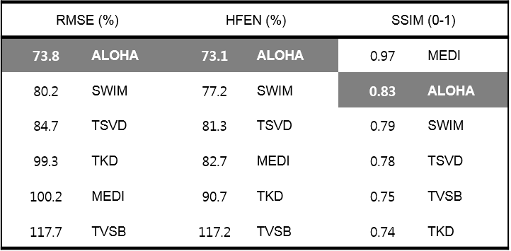
The proposed algorithm was compared with the conventional QSM dipole inversion methods. Numerical phantom data was downloaded online⁶ at http://weill.cornell.edu/mri/pages/qsm.html and in-vivo human brain data from QSM challenge 2016⁷ (http://qsm2016.com/) were also used. For quantitative comparison, we used three metrics⁷: root mean squared error (RMSE), high-frequency error norm (HFEN), structure similarity index (SSIM), which were also used for comparison in QSM Challenge 2016. COSMOS was assumed to be the ground truth. For numerical phantom and in-vivo human brain, optimization parameters were empirically determined by minimizing RMSE for each data.

Results and Discussion

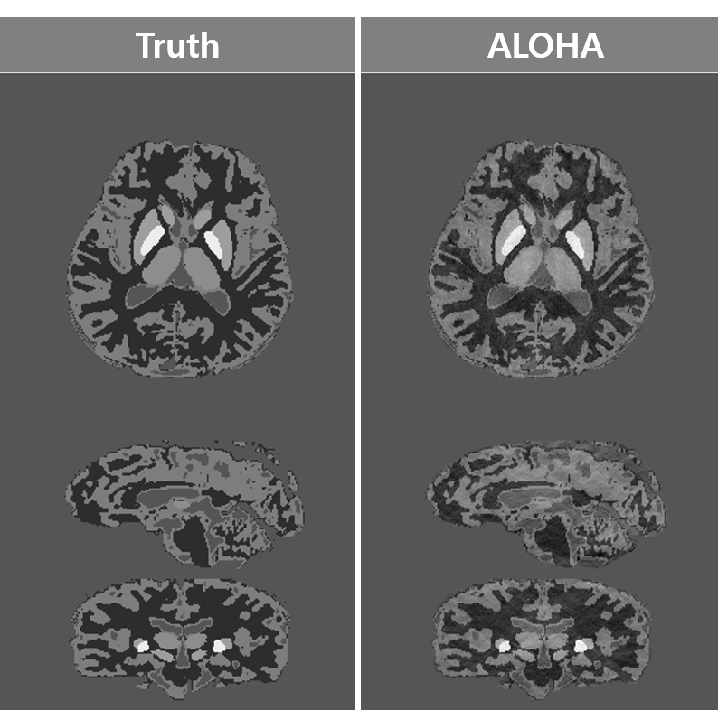
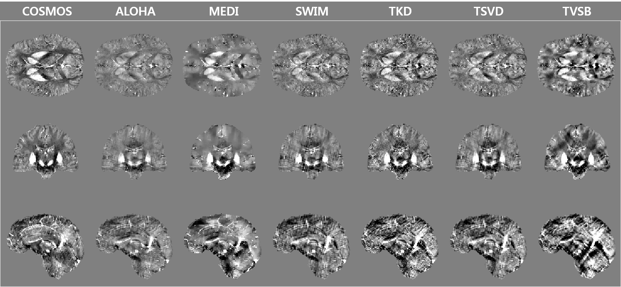
The parameter optimization results for phantom were $$$\lambda=10^{1.3},\mu=10^{-2.3},N_{1}=10,N_{2,3}=6$$$, and those for human data were $$$\lambda=10^{2},\mu=10^{-1.8},N_{1}=60,N_{2,3}=6$$$. Our proposed algorithm successfully reconstructed the susceptibility image from the phase image for the numerical phantom and human data (Figs.2 and 3). Specifically, our algorithm showed fine vascular structures without streaking artifacts on the coronal and sagittal slices. In addition, over-smoothing problem was not shown. Each methods were compared quantitatively (Table.1), and the proposed method showed superior performance over the existing methods.

Conclusion

Acknowledgements

References

[1] Wharton, S., & Bowtell, R. Whole-brain susceptibility mapping at high field: a comparison of multiple-and single-orientation methods. Neuroimage, 2010; 53(2), 515-525.

[2] Shmueli, K., de Zwart, J. A., van Gelderen, P., Li, T. Q., Dodd, S. J., & Duyn, J. H. Magnetic susceptibility mapping of brain tissue in vivo using MRI phase data. Magnetic Resonance in Medicine ,2009; 62(6), 1510-1522.

[3] Liu, J., Liu, T., de Rochefort, L., Ledoux, J., Khalidov, I., Chen, W., . . . Prince, M. R. Morphology enabled dipole inversion for quantitative susceptibility mapping using structural consistency between the magnitude image and the susceptibility map. Neuroimage, 2012; 59(3), 2560-2568.

[4] Wu, B., Li, W., Guidon, A., & Liu, C. Whole brain susceptibility mapping using compressed sensing. Magnetic Resonance in Medicine, 2012; 67(1), 137-147

[5] Jin, K. H., Lee, D., & Ye, J. C. A general framework for compressed sensing and parallel MRI using annihilating filter based low-rank Hankel matrix. IEEE Transactions on Computational Imaging 2016; 2(4), 480-495.

[6] Wang, Y., & Liu, T. Quantitative susceptibility mapping (QSM): decoding MRI data for a tissue magnetic biomarker. Magnetic Resonance in Medicine, 2015; 73(1), 82-101

[7] Langkammer, C., Schweser, F., Shmueli, K., Kames, C., Li, X., Guo, L., . . . Bredies, K Quantitative susceptibility mapping: Report from the 2016 reconstruction challenge. Magnetic Resonance in Medicine, 2017;