2198

DeepQSM - Solving the Quantitative Susceptibility Mapping Inverse Problem Using Deep Learning

Mads Kristensen¹, Kasper Gade Bøtker Rasmussen¹, Rasmus Guldhammer Blendal¹, Lasse Riis Østergaard¹, Maciej Plocharski¹, Andrew Janke², Christian Langkammer³, Kieran O’Brien^2,4, Markus Barth², and Steffen Bollmann²

¹Department of Health Science and Technology, Aalborg University, Aalborg, Denmark, ²Centre for Advanced Imaging, University of Queensland, Brisbane, Australia, ³Department of Neurology, Medical University of Graz, Graz, Austria, ⁴Siemens Healthcare Pty Ltd, Brisbane, Australia

Synopsis

Quantitative susceptibility mapping (QSM) aims to extract the magnetic susceptibility of tissue by solving an ill-posed field-to-source-inversion. Current QSM algorithms require manual parameter choices to balance between smoothing, artifacts and quantitation accuracy. Deep neural networks have been shown to perform well on ill-posed problems and can find optimal parameter sets for a given problem based on real-world training data. We have developed a proof-of-concept fully convolutional deep network capable of solving QSM’s ill-posed field-to-source inversion that preserves fine spatial structures and delivers accurate quantitation results.

Introduction

Quantitative susceptibility mapping (QSM), is a post processing technique that aims to quantify the magnetic susceptibility of tissue¹. It has potential to give new and unique, non-invasive insight into neurodegenerative disease pathology and differentiate between different types of lesions in the brain^2–5. In order to compute the field-to-source-inversion an ill-posed deconvolution is required from magnetic field phase data to susceptibility source of the local tissues⁶. The current gold standard COSMOS (Calculation of susceptibility through multiple orientation sampling) uses signal phase obtained from multiple head orientations to stabilize the inverse problem⁷, but the method is not clinically feasible due to time constraints and patient discomfort^1,8. A range of methods exist to solve the inverse problem from single-orientation 3D phase data, such as truncated k-space division (TKD⁹), morphology enabled dipole inversion (MEDI¹⁰), total generalized variation (TGV¹¹), single-step QSM (SS-QSM¹²) or sparse linear equation and least-squares algorithms (LSQR¹³). Despite their good performance on error metrics, the resulting images often show a significant amount of smoothing and artifacts due to the regularizations applied. The regularization parameters need to be carefully chosen to yield a trade-off between artifacts, smoothing and quantitation accuracy. Neural networks have been shown to perform well on ill-posed problems and can optimize a large amount of parameters for a given problem based on a large amount of training data^14–18. We therefore hypothesize that a fully convolutional deep network could solve QSM’s ill-posed field-to-source inversion while preserving fine spatial structures and delivering accurate quantitation results. To the best of our knowledge, neural networks have not been applied to the QSM field-to-source problem and we show a first proof-of-concept by attempting to invert a convolution using a two-dimensional dipole kernel.

Methods

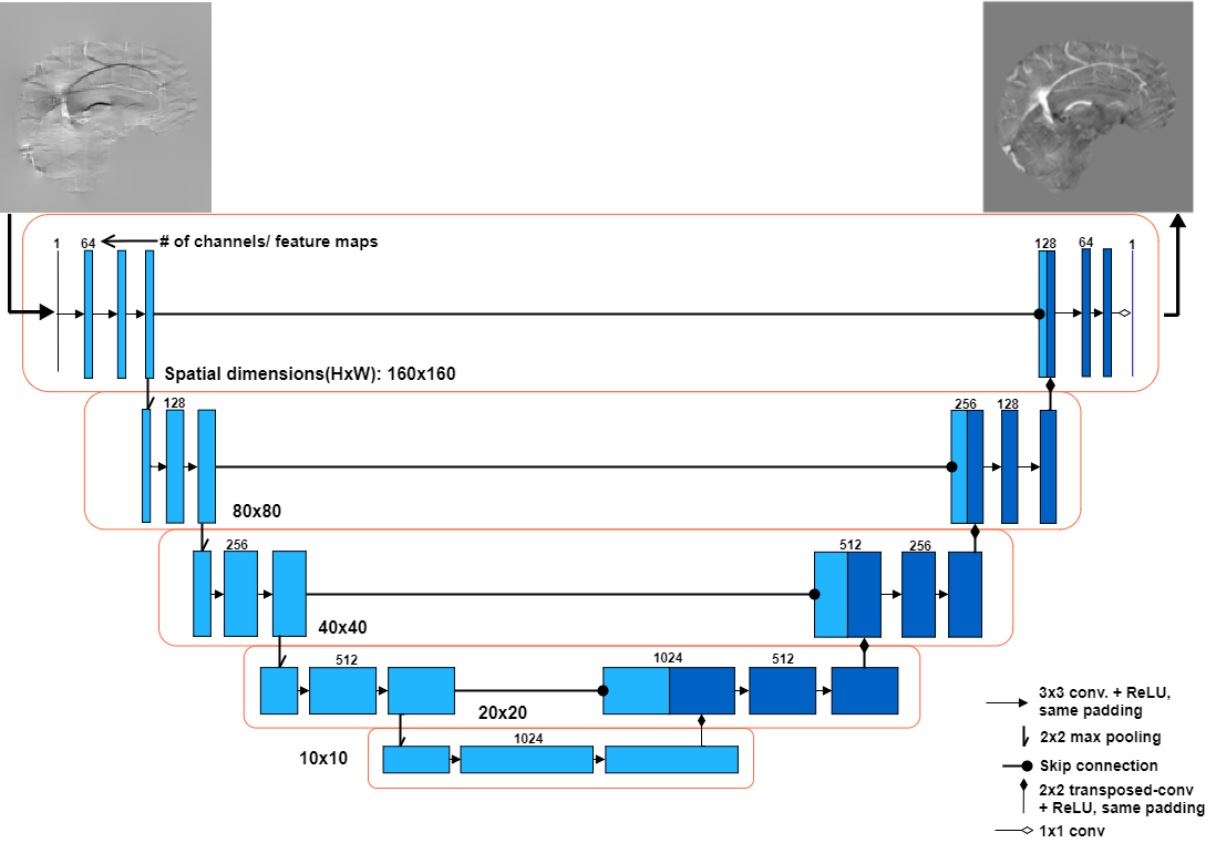
The fully convolutional neural network (DeepQSM) is based on U-NET¹⁹, as the architecture has proven to be efficient with inverse problems¹⁵. The full architecture is shown in Figure 1. DeepQSM was implemented in Python 3.6 using Tensorflow v1.3²⁰ and was trained in 32 hours on an Nvidia Tesla K40c with simulated examples of size 160x160 pixels and a batch size of 64 examples for 15 epochs training on 1600 batches of example data per epoch. The simulated training dataset consisted of basic geometric shapes such as squares, rectangles and circles of random size, occurrence and overlap with randomly assigned susceptibilities. The simulated susceptibility distribution was convolved with the 2D dipole kernel and white Gaussian noise with SNR of 50dB was added to generate tissue phase data. No MR image data was used to train the network to ensure it learned the general concept behind the field-to-source inversion for QSM. To test the network’s generalizability, we convolved the COSMOS reconstruction from the 2016 Reconstruction Challenge⁸ with the dipole kernel to generate tissue phase and used this as an input for the network to predict the underlying susceptibility distribution. We compared the prediction of the network to the COSMOS ground-truth and a TKD reconstruction. The results were quantitatively evaluated using three error metrics⁸: root-mean-square error (RMSE), high-frequency error norm (HFEN) and structural similarity index (SSIM).

Results and discussion

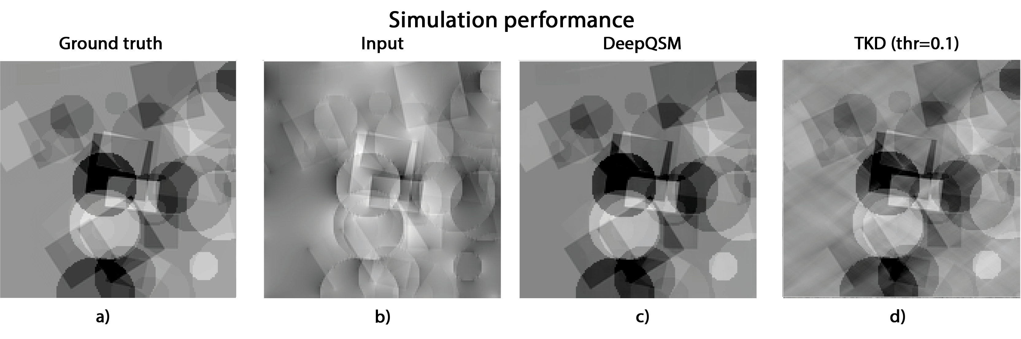
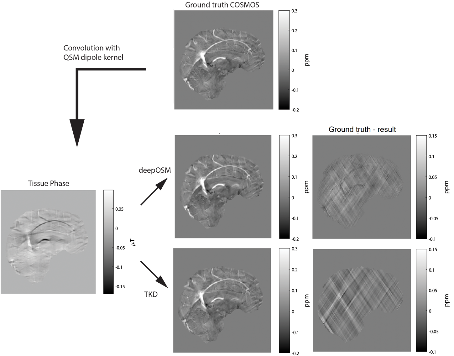
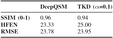
The output of DeepQSM on simulated data, see Figure 2, shows minimal differences to the ground truth. Error metrics obtained for DeepQSM and TKD (α=0.1) can be seen in Table 1. The DeepQSM network successfully learned to solve the general inverse problem, as shown in Figure 3. Figure 3 illustrates the network’s output, which is nearly identical to the ground truth, and shows considerably reduced streaking artifacts compared to TKD (α=0.1). The current proof-of-concept implementation already shows promising results by utilizing a simplified two dimensional version of the dipole kernel, but the presented deep learning approach is capable of utilizing any forward model and as such could potentially incorporate background field correction and additional model terms accounting for anisotropy of magnetic susceptibility and structural tissue anisotropy²¹. Further, DeepQSM does not require explicit sparsity or smoothness assumptions in order to suppress streaking artifacts, but finds a parameter set based on the training data and cost function. It therefore has the potential to better preserve the fine detailed anatomical structures.

Conclusion

DeepQSM learned to solve the inverse problem and can successfully apply the inverse operation of the dipole kernel on arbitrary images. The predicted susceptibility map yields comparable results to the simulated data, showing that the network generalized the dipole inversion. We therefore present a proof-of-concept convolutional neural network that can propose a solution to the ill-posed inversion from magnetic field phase data to susceptibility source.

Acknowledgements

The authors acknowledge the facilities of the National Imaging Facility at the Centre for Advanced Imaging, University of Queensland. The three first authors acknowledge funding from the following private organisations: Aalborg University Internationalisation foundation, Otto Mønsted foundation, Knud Højgaard foundation, Danish Tennis Foundation, Nordea foundation, Julie Damms study-foundation and Oticon foundation. SB acknowledges funding from UQ Postdoctoral Research Fellowship grant and support via an NVIDIA hardware grant. This research/project was undertaken with the assistance of resources and services from the National Computational Infrastructure (NCI), which is supported by the Australian Government.

References

1. Deistung, A., Schweser, F. & Reichenbach, J. R. Overview of quantitative susceptibility mapping: Overview of Quantitative Susceptibility Mapping. NMR Biomed. 30, e3569 (2017).

2. Deistung, A. et al. Toward in vivo histology: A comparison of quantitative susceptibility mapping (QSM) with magnitude-, phase-, and R2⁎-imaging at ultra-high magnetic field strength. NeuroImage 65, 299–314 (2013).

3. Liu, C., Li, W., Tong, K. A., Yeom, K. W. & Kuzminski, S. Susceptibility-weighted imaging and quantitative susceptibility mapping in the brain: Brain Susceptibility Imaging and Mapping. J. Magn. Reson. Imaging 42, 23–41 (2015).

4. Chen, W. et al. Intracranial calcifications and hemorrhages: characterization with quantitative susceptibility mapping. Radiology 270, 496–505 (2014).

5. Li, W. et al. Differential developmental trajectories of magnetic susceptibility in human brain gray and white matter over the lifespan: Brain Magnetic Susceptibility Over Lifespan. Hum. Brain Mapp. 35, 2698–2713 (2014).

6. Schweser, F., Deistung, A. & Reichenbach, J. R. Foundations of MRI phase imaging and processing for Quantitative Susceptibility Mapping (QSM). Z. Für Med. Phys. 26, 6–34 (2016).

7. Liu, T., Spincemaille, P., de Rochefort, L., Kressler, B. & Wang, Y. Calculation of susceptibility through multiple orientation sampling (COSMOS): A method for conditioning the inverse problem from measured magnetic field map to susceptibility source image in MRI. Magn. Reson. Med. 61, 196–204 (2009).

8. Langkammer, C. et al. Quantitative susceptibility mapping: Report from the 2016 reconstruction challenge. Magn. Reson. Med. n/a-n/a (2017). doi:10.1002/mrm.26830

9. Shmueli, K. et al. Magnetic susceptibility mapping of brain tissue in vivo using MRI phase data. Magn. Reson. Med. 62, 1510–1522 (2009).

10. Liu, T. et al. Morphology enabled dipole inversion (MEDI) from a single-angle acquisition: Comparison with COSMOS in human brain imaging. Magn. Reson. Med. 66, 777–783 (2011).

11. Langkammer, C. et al. Fast quantitative susceptibility mapping using 3D EPI and total generalized variation. NeuroImage 111, 622–630 (2015).

12. Chatnuntawech, I. et al. Single-step quantitative susceptibility mapping with variational penalties. NMR Biomed. n/a-n/a (2016). doi:10.1002/nbm.3570

13. Li, W. et al. A method for estimating and removing streaking artifacts in quantitative susceptibility mapping. NeuroImage 108, 111–122 (2015).

14. Dong, C., Deng, Y., Change Loy, C. & Tang, X. Compression artifacts reduction by a deep convolutional network. in Proceedings of the IEEE International Conference on Computer Vision 576–584 (2015).

15. Jin, K. H., McCann, M. T., Froustey, E. & Unser, M. Deep Convolutional Neural Network for Inverse Problems in Imaging. IEEE Trans. Image Process. 26, 4509–4522 (2017).

16. McCann, M. T., Jin, K. H. & Unser, M. A review of Convolutional Neural Networks for inverse problems in imaging. ArXiv Prepr. ArXiv171004011 (2017).

17. Golkov, V. et al. q-Space Deep Learning: Twelve-Fold Shorter and Model-Free Diffusion MRI Scans. IEEE Trans. Med. Imaging 35, 1344–1351 (2016).

18. Zhu, B., Liu, J. Z., Rosen, B. R., & Rosen, M. S. (2017). Image reconstruction by domain transform manifold learning. ArXiv:1704.08841 [Cs]. Retrieved from http://arxiv.org/abs/1704.08841

19. Ronneberger, O., Fischer, P. & Brox, T. U-Net: Convolutional Networks for Biomedical Image Segmentation. in Medical Image Computing and Computer-Assisted Intervention – MICCAI 2015 234–241 (Springer, Cham, 2015). doi:10.1007/978-3-319-24574-4_28

20. Abadi, M. et al. Tensorflow: Large-scale machine learning on heterogeneous distributed systems. ArXiv Prepr. ArXiv160304467 (2016).

21. Yablonskiy, D. A. & Sukstanskii, A. L. Generalized Lorentzian Tensor Approach (GLTA) as a biophysical background for quantitative susceptibility mapping. Magn. Reson. Med. 73, 757–764 (2015).

Figures

Fig. 1. DeepQSM architecture based on U-NET^15,19. Input data is a 160x160 image, and the network consists of 3x3 convolutions, with same padding, 2x2 pooling on one side, and 2x2 up convolutions on the other side. The transposed convolutions undo the pooling operation, and skip connections are used for residual learning. The final convolution is a 1x1 to reduce the feature maps to 1 and to achieve an MxN output image.

Fig. 2. DeepQSM’s performance on simulated data. a) simulated susceptibility distribution. b) simulated tissue phase data. c) the prediction of the network. d) shows a truncated k-space division (TKD) solution for comparison. Notice how DeepQSM is very similar to the ground truth but TKD suffers from streaking artifacts.

Fig. 3. The “calculation of susceptibility through multiple orientation sampling” (COSMOS) image was convolved with the dipole kernel to create a tissue phase image. The same tissue phase image was used as input to the DeepQSM neural network and the truncated k-space division (TKD) algorithm (α=0.1). Lastly difference maps were created by subtracting DeepQSM prediction from the COSMOS image and another by subtracting the TKD result from the COSMOS image.

Table 1: Error metrics of results from DeepQSM and TKD. RMSE (Root Mean Square Error). SSIM (Structural Similarity Index) is a combined measure obtained from three complementary components (luminance similarity, contrast similarity, and structural similarity)⁸. HFEN (High Frequency Error Norm) aims to measure the fidelity at high spatial frequencies⁸.

Proc. Intl. Soc. Mag. Reson. Med. 26 (2018)

2198