2191
Evaluating the Precision of Multi-Echo Combination Methods for Susceptibility Mapping by Analysing the Propagation of Single-Echo Phase Noise into Multi-Echo Field and Susceptibility Maps1Medical Physics and Biomedical Engineering, University College London, London, United Kingdom, 2Academic Neuroradiological Unit, Department of Brain Repair and Rehabilitation, Institute of Neurology, University College London, London, United Kingdom, 3Leonard Wolfson Experimental Neurology Centre, Institute of Neurology, University College London, London, United Kingdom
Synopsis
In Susceptibility Mapping (SM) using multi-echo acquisitions, noise propagates from the single-echo phase images into the field map in a manner dependent on the method used for multi-echo combination. Field noise then propagates into the susceptibility map, determining the precision of the measured susceptibility. Here, we characterised the propagation of single-echo phase noise into both the combined field and susceptibility maps using three methods for multi-echo combination: fitting, averaging and echo time-weighted averaging. We calculated susceptibility noise maps for both simulated and acquired data, showing that, when choosing a pipeline for multi-echo SM, it is important to consider its precision.
Introduction
Accuracy and precision are two metrics that enable the full characterisation of a processing pipeline for susceptibility mapping (SM). A pipeline’s accuracy depends on the closeness of the measured susceptibility $$$\chi$$$ to $$$\chi$$$’s true value, whereas its precision is determined by how the noise propagates from the signal phase into the measured $$$\chi$$$.
In previous studies of SM of multi-echo gradient-echo (GRE) images1,2, we showed that combining multiple echoes by non-linearly fitting the complex GRE signal over echo times (TEs) (NLFit) gives a more accurate average $$$\chi$$$ than combining multiple echoes by averaging the single-echo phase over TEs, both without weighting (Avg) or with weighting proportional to the TE (wAvg) (Figure 1). Here, we aimed to evaluate how the noise propagates from the single-echo phase images $$$\sigma(\phi(TE))$$$ into the total and local field ($$${\Delta}B_{Tot}$$$ and $$${\Delta}B_{Loc}$$$) and $$$\chi$$$.
We calculated the noise in a $$$\chi$$$ map $$$\sigma(\chi)$$$ as a function of $$$\sigma\left({\Delta}B_{Loc}\right)$$$ for $$$\chi$$$ calculated using Thresholded K-space Division (TKD)3. Previous studies using NLFit4 or Avg5 have calculated the noise in $$${\Delta}B_{Tot}$$$ ($$$\sigma({\Delta}B_{Tot})$$$), but an expression for $$$\sigma({\Delta}B_{Tot})$$$ has not yet been calculated for wAvg6,7 so we derived this here. We compared $$$\sigma({\Delta}B_{Loc})$$$ and $$$\sigma(\chi)$$$ in the three pipelines using data simulated from a realistic head phantom and images of five healthy volunteers (HVs).
Theory
The equations for the calculation of $$$\sigma\left({\Delta}B_{Tot}\right)$$$, including the one we derived for wAvg, are shown at the bottom of Figure 1, with $$$n$$$ the number of TEs and $$$\sigma^2$$$ the variance.
For all pipelines, based on error propagation and the orthogonality8 of $$${\Delta}B_{Loc}$$$ and the background fields ($$${\Delta}B_{Bg}$$$) in the brain:
$$\sigma({\Delta}B_{Loc}(\mathbf{r}))=\sqrt{\sigma^2({\Delta}B_{Tot}(\mathbf{r}))-\sigma^2({\Delta}B_{Bg}(\mathbf{r}))}\qquad[1]$$
with $$$\mathbf{r}$$$ the position of a voxel in image space. Thus,
$$\sigma({\Delta}B_{Loc}(\mathbf{r}))\leq\sigma({\Delta}B_{Tot}(\mathbf{r}))\qquad[2]$$
Based on error propagation, the worst-case noise in $$$\chi$$$ for TKD3 is:
$$\sigma(\chi(\mathbf{r}))=\frac{\sqrt{FT^{-1}(D^{-2}\left(\mathbf{k}\right)FT\left(\sigma^2\left({\Delta}B_{Tot}\left(\mathbf{r}\right)\right)\right)}}{B_0}\qquad[3]$$
with $$$D$$$ the TKD dipole kernel in k-space, $$$\mathbf{k}$$$ the position of a voxel in k-space, $$$FT$$$ the Fourier Transform and $$$B_0$$$ the field strength.
Methods
Multi-echo 3D GRE brain images of five HVs were acquired on a Philips Achieva 3T system (Best, NL) using a 32-channel head coil and a previously described protocol9. Two data sets were acquired in the same session, with $$$M_i,\phi_i$$$ for $$$i=1,2$$$ the magnitude and phase from each data set.
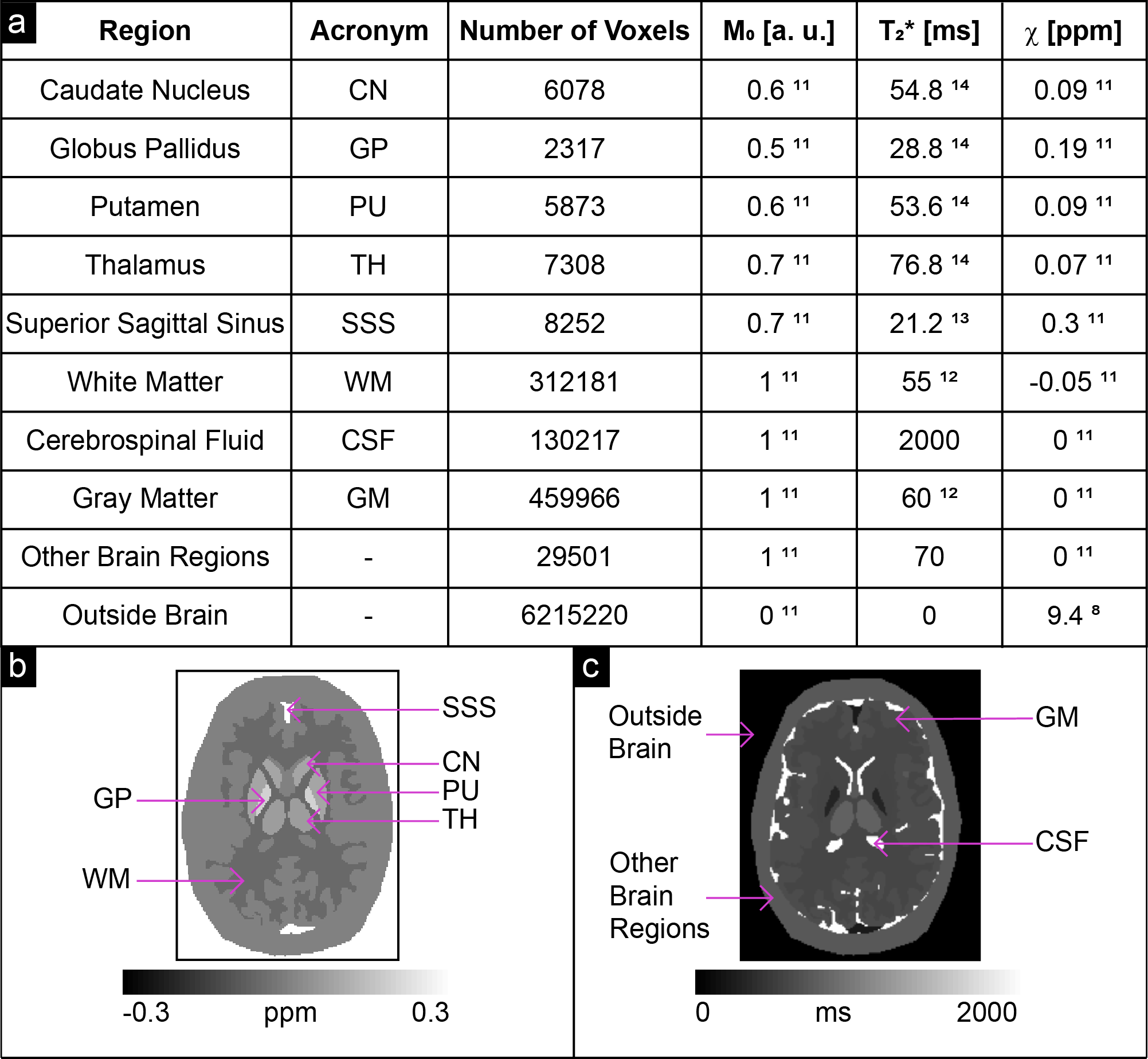
Noisy complex data were simulated at the same TEs, at 3 T, based on a Zubal head phantom10 using realistic ground-truth $$$\chi$$$8,11, proton density ($$$M_0$$$)11 and $$$T_2^*$$$ values12-14 (Figure 2), and a standard deviation (SD) of the magnitude $$$\sigma(M)=0.07$$$ chosen according to the following magnitude signal-to-noise ratio (SNR) criterion for the longest TE image15 in the superior sagittal sinus (SSS):
$$\min_{TE}\left(SNR\right)\geq3{\quad\Leftrightarrow\quad}\sigma(M)\leq\frac{M_{0,SSS}(TE_5)\exp(-TE_5/T_{2,SSS}^*)}{3}=\frac{0.7\exp(-24.6ms/21.2ms)}{3}=0.07\qquad[4]$$
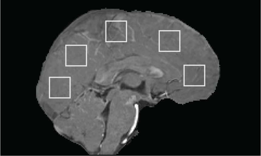
Five 20x20-voxel ROIs16 were drawn on a sagittal slice of HV1’s first-echo $$$M_1$$$ image (Figure 3), then copied to $$$M_1$$$ of HV2-5 after rigid image co-registration with NiftyReg17.
In each HV, ROI-based magnitude ($$$M_{ROI}$$$), magnitude noise ($$$\sigma_{ROI}(M)$$$) and phase noise ($$$\sigma_{ROI}(\phi)$$$) values were calculated as18:
$$M_{ROI}(TE,\mathbf{r})=\frac{1}{2}mean(M_1(TE,\mathbf{r}+M_2(TE,\mathbf{r}))),\quad\mathbf{r}\in\text{ROI}\qquad[5]$$
$$\sigma_{ROI}(M(TE,\mathbf{r}))=\sqrt{R}\frac{1}{\sqrt{2}}SD(M_1(TE,\mathbf{r})-M_2(TE,\mathbf{r})),\quad\mathbf{r}\in\text{ROI}\qquad[6]$$
$$\sigma_{ROI}(\phi(TE,\mathbf{r}))=\sqrt{R}\frac{1}{\sqrt{2}}SD(\phi_1(TE,\mathbf{r})-\phi_2(TE,\mathbf{r})),\quad\mathbf{r}\in\text{ROI}\qquad[7]$$
with $$$R$$$ the 2D-SENSE reduction factor19. Equations [5]-[7] were averaged across ROIs to create summary values of magnitude ($$$\hat{M}_{ROI}$$$), magnitude noise ($$$\hat{\sigma}_{ROI}(M)$$$) and phase noise ($$$\hat{\sigma}_{ROI}(\phi)$$$) at each TE.
For both the simulations and the HVs, a map of $$$\mathbf{\sigma(\phi)}$$$ was calculated at each TE as15:
$$\sigma(\phi(TE,\mathbf{r}))=c(TE)\frac{1}{SNR(TE,\mathbf{r})}=c(TE)\frac{\hat{\sigma}_{ROI}(M(TE))}{M(TE,\mathbf{r})}\qquad[8]$$
with $$$c$$$ a constant of proportionality equal to 1 in the simulations and to
$$c(TE)=\frac{\hat{\sigma}_{ROI}(\phi(TE))}{1/SNR_{ROI}(M)}=\frac{\hat{\sigma}_{ROI}(\phi(TE))\hat{\sigma}_{ROI}(M(TE))}{\hat{M}_{ROI}(TE)}\qquad[9]$$
in the HVs.
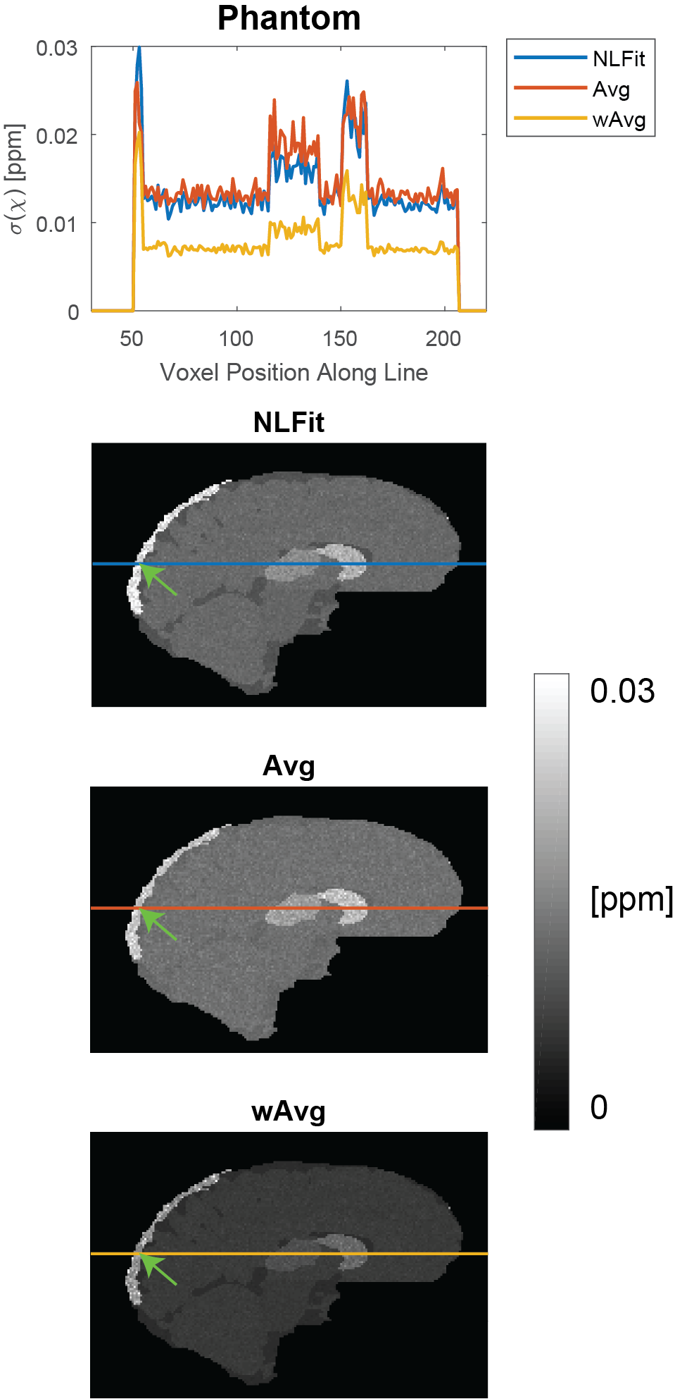
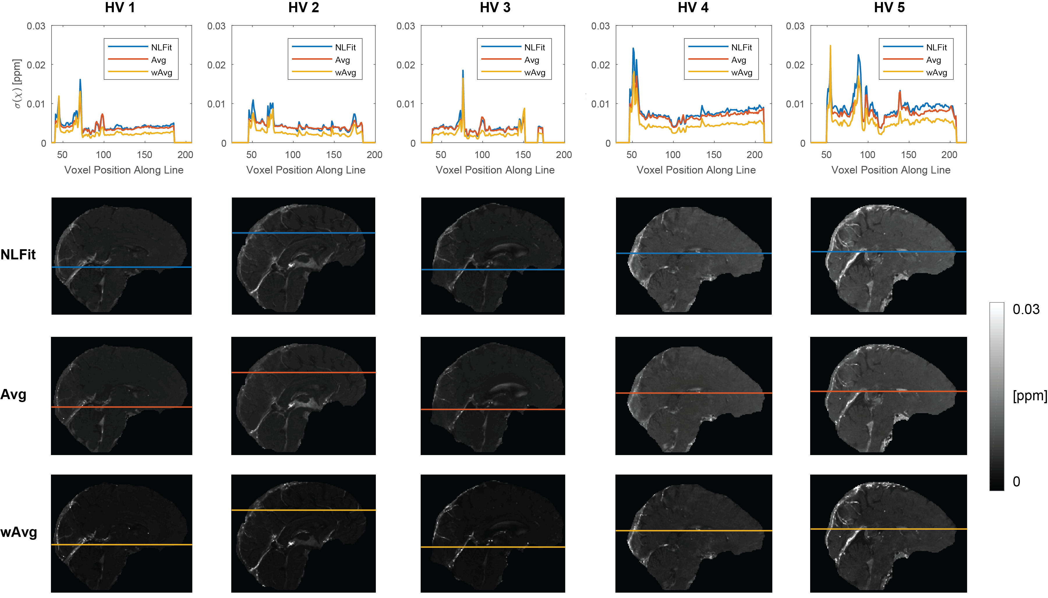
For each pipeline, a map of $$$\sigma({\Delta}B_{Tot})$$$ was calculated from the multi-echo $$$\sigma(\phi)$$$ maps using the corresponding equation for $$$\sigma({\Delta}B_{Tot})$$$ (Figure 1, F1-F3). Then, $$$\sigma(\chi)$$$ was calculated using Eq. [3] with $$$\sigma({\Delta}B_{Tot})$$$ for the corresponding pipeline, a threshold=2/3 for $$$D$$$'s inversion, and correction for $$$\chi$$$ underestimation20. To compare $$$\sigma({\Delta}B_{Tot})$$$ and $$$\sigma(\chi)$$$ between pipelines a line profile was traced in the $$$\sigma({\Delta}B_{Tot})$$$ and $$$\sigma(\chi)$$$ images.
Results and Discussion
In both the phantom (Figure 4) and the HVs (Figure 5), wAvg had the lowest $$$\sigma(\chi)$$$, whereas Avg and NLFit had a similar $$$\sigma(\chi)$$$. In both the phantom and the HVs, the difference between NLFit and wAvg/Avg appeared prominent in large-$$$\chi$$$ regions, in line with our previous studies1,2, where $$$\chi$$$ calculated by wAvg always had the smallest SD in all ROIs and $$$\chi$$$ calculated by NLFit always had the largest SD in the veins. $$$\sigma(\chi)$$$ differences between different pipelines, however, were always in the order of a few parts per billion.
Conclusions
We have shown that for multi-echo SM combining the multi-echo phase by fitting vs. averaging over TEs is less precise, although it is more accurate in high-$$$\chi$$$ regions1,2. We suggest that the precision and accuracy of $$$\chi$$$ should be analysed together to assess and compare the relative performance of different SM pipelines for different applications.Acknowledgements
DLT is supported by the UCL Leonard Wolfson Experimental Neurology Centre (PR/ylr/18575).References
- Biondetti E, Thomas D L and Shmueli K. Application of Laplacian-based Methods to Multi-Echo Phase Data for Accurate Susceptibility Mapping. Proceedings of the International Society for Magnetic Resonance in Medicine. 2016; 24:1547.
- Biondetti E, Karsa A, Thomas D L, et al. The Effect of Averaging the Laplacian-Processed Phase over Echo Times on the Accuracy of Local Field and Susceptibility Maps. Graz, Austria: 4th International Workshop on MRI Phase Contrast & Quantitative Susceptibility Mapping; 2016.
- Shmueli K, de Zwart JA, van Gelderen P, et al. Magnetic susceptibility mapping of brain tissue in vivo using MRI phase data. Magnetic Resonance in Medicine. 2009;62(6):1510–1522.
- Kressler B, De Rochefort L, Liu T, et al. Nonlinear regularization for per voxel estimation of magnetic susceptibility distributions from MRI field maps. IEEE Transactions on Medical Imaging. 2010;29(2):273–281.
- Wu B, Li W, Avram AV, et al. Fast and tissue-optimized mapping of magnetic susceptibility and T2* with multi-echo and multi-shot spirals. NeuroImage. 2012;59(1):297–305.
- Li W, Wang N, Yu F, et al. A method for estimating and removing streaking artifacts in quantitative susceptibility mapping. NeuroImage. 2015;108:111–122.
- Wei H, Dibb R, Zhou Y, et al. Streaking artifact reduction for quantitative susceptibility mapping of sources with large dynamic range. NMR in Biomedicine. 2015;28(10):1294–1303.
- Liu T, Khalidov I, de Rochefort L, et al. A novel background field removal method for MRI using projection onto dipole fields (PDF). NMR in Biomedicine. 2011;24(9):1129–1136.
- Biondetti E, Karsa A, Thomas DL, et al. Evaluating The Accuracy of Susceptibility Maps Calculated from Single-Echo versus Multi- Echo Gradient-Echo Acquisitions. Proceedings of the International Society of Magnetic Resonance in Medicine. 2017;25:1955.
- Zubal IG, Harrell CR, Smith EO, et al. Two dedicated software, voxel-based, anthropomorphic (torso and head) phantoms. Proceeding of the International Conference at the National Radiological Protection Board. 1995:105–111.
- Liu T, Wisnieff C, Lou M, et al. Nonlinear formulation of the magnetic field to source relationship for robust quantitative susceptibility mapping. Magnetic Resonance in Medicine. 2013;69(2):467–476.
- Peters AM, Brookes MJ, Hoogenraad FG, et al. T2* measurements in human brain at 1.5, 3 and 7 T. Proceedings of the International Society for Magnetic Resonance in Medicine 2006;14:926.
- Zhao JM, Clingman CS, Närväinen MJ, et al. Oxygenation and hematocrit dependence of transverse relaxation rates of blood at 3T. Magnetic Resonance in Medicine. 2007;58(3):592–597.
- Yao B, Li T-Q, van Gelderen P, et al. Susceptibility contrast in high field MRI of human brain as a function of tissue iron content. NeuroImage. 2009;44(4):1259–1266.
- Gudbjartsson H and Patz S. The Rician distribution of noisy MRI data. Magnetic Resonance in Medicine. 1995;34(6):910–914.
- Lerski RA, de Wilde J, Boyce D, et al. Quality Control in Magnetic Resonance Imaging. IPEM Report 80. York, UK: The Institute of Physics and Engineering in Medicine, 1998:14-16.
- Ourselin S, Roche A, Subsol G, et al. Reconstructing a 3D structure from serial histological sections. Image and Vision Computing. 2001;19(1–2):25–31.
- Dietrich O, Raya JG, Reeder SB, et al. Measurement of signal-to-noise ratios in MR images: Influence of multichannel coils, parallel imaging, and reconstruction filters. Journal of Magnetic Resonance Imaging. 2007;26(2):375–385.
- Weiger M, Pruessmann KP and Boesiger P. 2D SENSE for faster 3D MRI. Magnetic Resonance Materials in Physics, Biology and Medicine. 2002;14(1):10–19.
- Schweser F, Deistung A, Sommer K, et al. Toward online reconstruction of quantitative susceptibility maps: Superfast dipole inversion. Magnetic Resonance in Medicine. 2013;69(6):1582–1594.
Figures
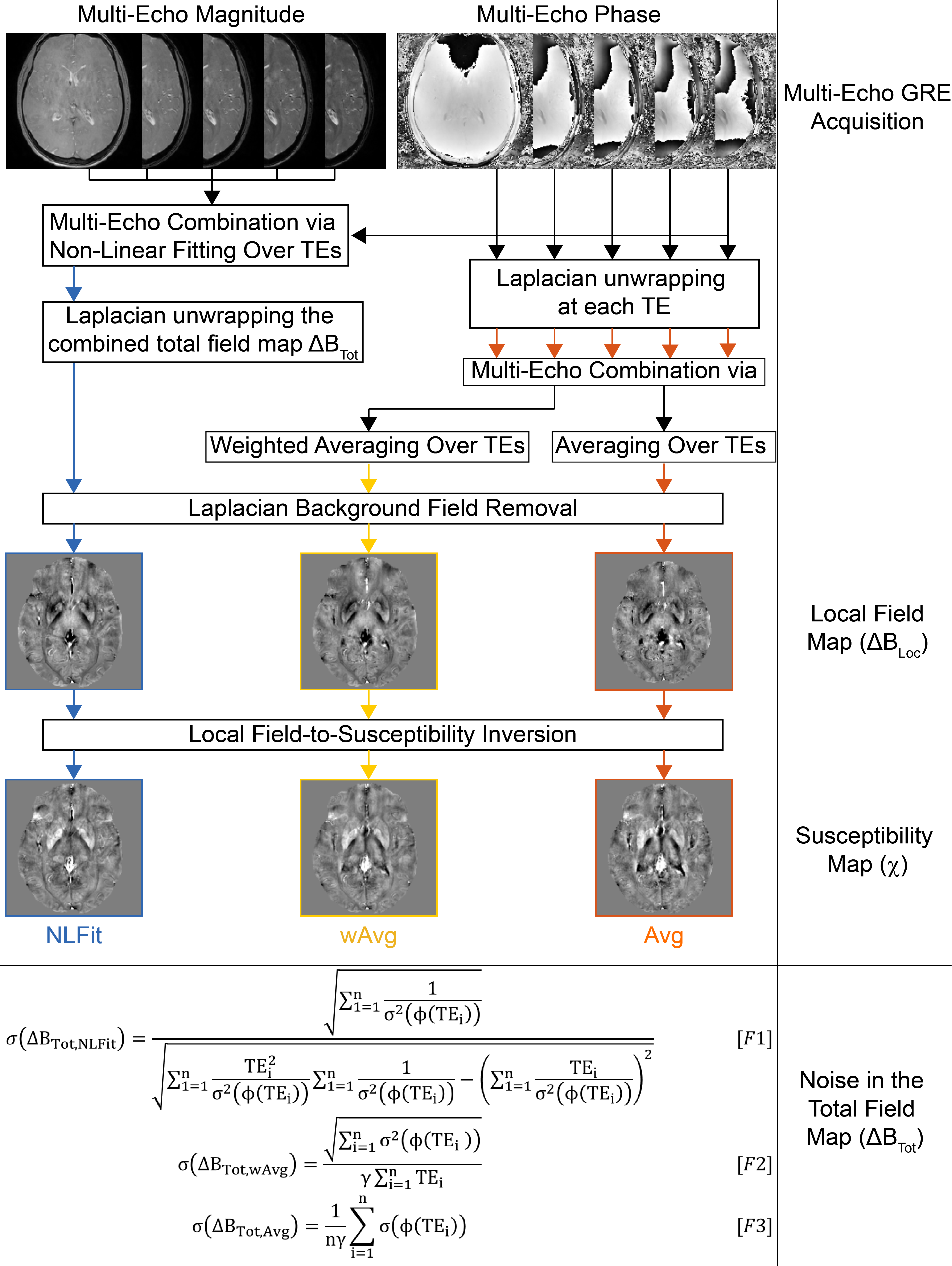
Figure 1 Processing pipelines for multi-echo SM analysed in this study. NLFit (blue) combines multiple TEs by non-linearly fitting the multi-echo complex signal over time11. wAvg (yellow) and Avg (orange) unwrap the single-echo phase using a Laplacian-based method (SHARP20 with a threshold=10-10) then combine multiple TEs by averaging5 (Avg) or averaging6,7 using a TE-based weighting of the phase (wAvg). All the pipelines remove background field variations from $$${\Delta}B_{Tot}$$$ using SHARP20 with a threshold=0.05, then calculate $$$\chi$$$ using TKD3 with correction for $$$\chi$$$ underestimation20.
In the bottom panel, the equations for the calculation of $$${\Delta}B_{Tot}$$$ are shown for each pipeline.