2182
Incorporating Bolus Arrival Time Offset into Fast Linear Analysis Could Shorten Acquisition Times for DCE-MRI1Brigham and Women's Hospital, Boston, MA, United States
Synopsis
Linearization of the Kety/Tofts model for DCE analysis drastically shortens computation time. We show that addition of bolus arrival time (BAT) compensation to the linearized analysis could also allow quicker acquisition times. With BAT inclusion, 3 minute sequences yield equivalent parameter estimation accuracy to 5 minute sequences without BAT compensation. The combination of shorter acquisition and real-time analysis would reduce the general time burden of DCE, which has potential implications for increased patient turnaround, and making DCE more acceptable as a tool, for example in evaluating response to therapy or in image guided therapy.
INTRODUCTION
Dynamic Contrast-Enhanced (DCE) MRI can potentially extract information about the tissue microstructure, vascularity and neovascularity, and underlying pathology. DCE data acquisition typically takes 5 minutes or more, and requires lengthy computational analysis via curve fitting to a pharmacokinetic model.
A critical component necessary for DCE analysis is the concentration of contrast agent in the blood entering the tissue of interest, which is often calculated from a region of interest covering a large artery in the acquired images. Since the average time for blood to travel once around the body is 20 sec, the arrival of contrast agent in the tissue is often delayed compared to the large artery. Ignoring the delay, also referred to as the bolus arrival time (BAT), has been shown to degrade the fit quality in DCE modeling1, while incorporation of a BAT shift improves reproducibility of calculated model parameters2. Here we describe how BAT compensation may be incorporated into a fast linearized analysis method, and demonstrate its effectiveness in short acquisitions.
A popular model of contrast agent uptake is the Kety/Tofts model 3,4, often used for clinical data. The contrast agent concentration time course is:
$$v_e\frac{dC_e(t)}{dt}=K_{trans}[C_p(t)−C_e(t)]$$[1]
where $$$C_e(t)$$$ is the extracellular tissue concentration of contrast agent with $$$v_e$$$ being the fraction of the tissue that is extracellular, $$$C_p(t)$$$ is the blood plasma concentration of contrast agent, often referred to as the arterial input function (AIF), and $$$K_{trans}$$$ is the transfer constant between plasma and tissue extracellular space quantifying leakage between compartments. The parameters of interest, $$$K_{trans}$$$ and $$$v_e$$$, are usually found from time-consuming nonlinear fitting of tissue contrast time courses.
Linearization of the Kety/Tofts Equation has been shown to be a very fast method of extracting pharmacokinetic parameters from DCE data, particularly at low SNR5,6, achieving a factor of 6 improvement in computation time5. Linearization in this context consists of creating a set of linear equations by integrating both sides of Eq. 1 as follows:
$$C_t(t)=K_{trans}\int_{0}^{t}C_p(u)du-k_{ep}\int_{0}^{t}C_t(u)du$$[2]
where $$$k_{ep}=K_{trans}/v_e$$$, and $$$C_t(t)=v_e C_e(t)$$$ is the total tissue concentration of contrast agent.
METHODS: THEORY
If the AIF bolus arrives at the tissue of interest at time $$$t_0$$$ after it is detected in the arterial blood voxel, Eq. 2 becomes:
$$C_t(t)=K_{trans}\int_{0}^{t-t_0}C_p(u)du-k_{ep}\int_{0}^{t}C_t(u)du$$[3]
The continuous representation of concentration is measured as a sparsely sampled MR signal, i.e., images are generated at discrete timepoints $$$t_j\in\{t_1,t_2,...,t_n\}$$$ where the time between frames is $$$\Delta t=t_j-t_{j-1}$$$. Discretization of Eq. 3 results in the set of linear equations (one equation for each time point $$$t_j$$$), incorporating BAT for the 2-parameter Tofts Model:
$$C_t(t_j)=K_{trans}\left [\sum_{i=1}^{j}C_p(t_i)\Delta t-t_0C_p(t_j)\right ]-k_{ep}\sum_{i=1}^{j}C_t(t_i)\Delta t$$[4]
This set of equations can be solved very quickly in each voxel for $$$k_{trans}$$$ and $$$v_e$$$ (and $$$t_0$$$) by matrix inversion.
METHODS: SIMULATIONS
Digital reference objects (DRO) built to represent the DCE signal from typical prostate tissue and different pulse sequences with a range of values for the parameters $$$K_{trans}$$$, $$$v_e$$$, and $$$t_0$$$. The parameter values assigned were:
$$$K_{trans}\in [0.05, 0.1, 0.2, 0.3, 0.4]$$$,
$$$v_e\in [0.15, 0.25, 0.35]$$$,
$$$t_0\in[0, 2, 4]$$$.
The signal in the simulated AIF pixels shown in Figure 1 was created from the mean AIF from 7 patients in a recent prostate study7. The simulated T1-FLASH pulse sequence parameters that were varied were: volume acquisition time (or frame time $$$\Delta t$$$) 3 or 5 sec, and total acquisition time: 3 or 5 minutes. After generating 100 pixels for each combination of tissue parameters , random noise was added to each voxel and each time point.
RESULTS
Figure 2 shows a comparison of the accuracy of calculated values for $$$K_{trans}$$$ depending on the simulated pulse sequence used. When the simulated BAT is 2 sec there is no advantage to adding BAT to the computation but at BAT=4sec it is clear that addition of BAT improves the accuracy of $$$K_{trans}$$$ estimation. For $$$v_e$$$, shown in Figure 3, even when BAT=2s, addition of BAT improves the estimate, with a large improvement seen for short sequences of 3 minutes. When BAT=4sec, the improvements in the case of $$$v_e$$$ are even more pronounced.DISCUSSION AND CONCLUSIONS
Conventional non-linear curve-fitting pharmacokinetic DCE analysis is computationally intense and sensitive to initial seed values. The very fast linearized analysis method has been shown to fit the parameters equally well at low SNR, corresponding to typical DCE scans used clinically. Addition of a BAT parameter to the linearized analysis improves the fit in simulations when a BAT offset exists. Moreover, when BAT is added, the parameter estimates appears to be less sensitive to the length of the simulated data acquisition, yielding similar results for sequences of 3 minutes duration vs. 5 minutes duration. This raises the possibility of performing very short DCE acquisitions with very fast analysis in clinical settings.Acknowledgements
NIH U24 CA180918References
1. Mehrtash, A. et al. Bolus arrival time and its effect on tissue characterization with dynamic contrast-enhanced magnetic resonance imaging. J Med Imaging (Bellingham) 3, 014503 (2016).
2. Chouhan, M. D. et al. Estimation of contrast agent bolus arrival delays for improved reproducibility of liver DCE MRI. Phys. Med. Biol. 61, 6905–6918 (2016).
3. Kety, S. S. The theory and applications of the exchange of inert gas at the lungs and tissues. Pharmacol. Rev. 3, 1–41 (1951).
4. Tofts, P. S. & Kermode, A. G. Measurement of the blood-brain barrier permeability and leakage space using dynamic MR imaging. 1. Fundamental concepts. Magn. Reson. Med. 17, 357–367 (1991).
5. Murase, K. Efficient method for calculating kinetic parameters using T1-weighted dynamic contrast-enhanced magnetic resonance imaging. Magn. Reson. Med. 51, 858–862 (2004).
6. DeGrandchamp, J. B. et al. Predicting response before initiation of neoadjuvant chemotherapy in breast cancer using new methods for the analysis of dynamic contrast enhanced MRI (DCE MRI) data. in SPIE Medical Imaging 978811–978811–10 (International Society for Optics and Photonics, 2016).
7. Fedorov, A., Vangel, M. G., Tempany, C. M. & Fennessy, F. M. Multiparametric Magnetic Resonance Imaging of the Prostate: Repeatability of Volume and Apparent Diffusion Coefficient Quantification. Invest. Radiol. 52, 538–546 (2017).
8. Fennessy, F. M. et al. Practical considerations in T1 mapping of prostate for dynamic contrast enhancement pharmacokinetic analyses. Magn. Reson. Imaging 30, 1224–1233 (2012).
9. Lu, H., Clingman, C., Golay, X. & van Zijl, P. C. M. Determining the longitudinal relaxation time (T1) of blood at 3.0 Tesla. Magn. Reson. Med. 52, 679–682 (2004).
10. Fedorov, A. et al. 3D Slicer as an image computing platform for the Quantitative Imaging Network. Magn. Reson. Imaging 30, 1323–1341 (2012).
Figures
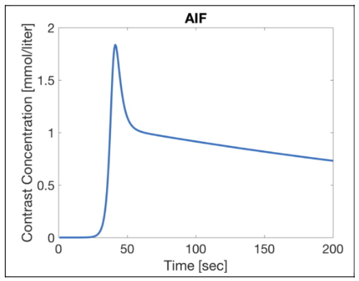
Simulated AIF extracted from the mean of measured AIF’s in a recent clinical prostate study. The AIF signal was discretized and included in each DRO and had the same noise added as the other voxels.
Relevant parameters held constant in the simulations were flip angle 15o , TR 5 ms, field strength (here 3T), contrast agent relaxivity (here 3.7 L/mmol sec) and hematocrit (here 0.45). T1 of tissue was simulated as 1434 ms 8, and the T1 of arterial blood was assumed to be 1630 ms 9.
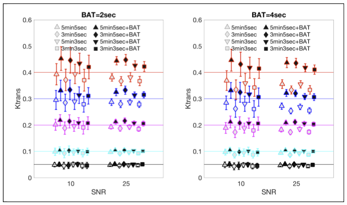
Comparison of $$$K_{trans}$$$ calculated with and without BAT compensation, vs. the original values used in creating the DROs for SNR=10 and SNR=25 and different pulse sequences.
The simulated DRO values of $$$K_{trans}$$$ are denoted by horizontal colored lines - each color corresponding to a different DRO value. Note that the final signal $$$S_{final}$$$ had a specified SNR: $$$S_{final}=\sqrt{(S+\eta)^2+\nu^2}$$$ where $$$S$$$ is the generated signal before noise addition and $$$\eta$$$ and $$$\nu$$$ are random numbers normally distributed around zero with standard deviation of SNR.
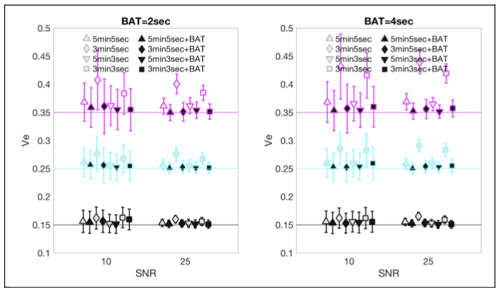
Comparison of $$$v_e$$$ calculated with and without BAT compensation, vs. the original values used in creating the DROs (horizontal colored lines), for SNR=10 and SNR=25.
Analysis was implemented in Matlab® (MATLAB Release 2016b, The MathWorks, Inc., Natick, MA, United States) utilizing the built in matrix inversion and using the 3D Slicer® version 4.6.2 (https://www.slicer.org)10 interface with the MatlabBridge Extension.