Synopsis

Background suppression is a recommended and frequently employed strategy to improve the perfusion-temporal-SNR (tSNR) of ASL. Since physiological signal fluctuations are known to be a major source of data corruption in functional MRI at higher magnetic field-strengths, it might also be expected that the benefits of BGS are even stronger at higher field-strengths. In this study, we evaluated and compared the importance of the introduction of BGS-pulses at 3T and 7T and show that, at higher magnetic field, BGS is even more crucial.

Introduction

Decreasing the static-tissue signal -and therefore reducing the physiological noise and motion artefacts- while preserving the ASL-signal is a recommended and frequently employed strategy to improve the perfusion-temporal-SNR (tSNR) of ASL¹. This so-called background-suppression (BGS) strategy consists in applying a series of inversion pulses to minimize the static-tissue signal at acquisition time^2,3. For MRI at higher magnetic field-strength, it is known that physiological signal fluctuations are a major source of data corruption in functional MRI⁴. It might therefore be expected that the benefits of BGS are even stronger at higher field-strengths. This might subsequently be an important argument to aim at 7T for readout approaches that exhibit optimal BGS over the complete imaging volume.

In this study, we evaluated and compared the importance of the introduction of BGS-pulses at 3T and 7T and show that, at higher magnetic field, BGS is even more crucial.

Methods

The same imaging protocol was carried out at 3T and 7T (Achieva, Philips, The Netherlands) using 32-channel head-coils. Seven and five subjects were scanned respectively at 7T and 3T. All subjects provided written informed consent for this IRB-approved study.

Labeling-Flow-alternating-inversion-recovery (FAIR) labeling was implemented consisting of a frequency-offset-corrected-inversion (FOCI) RF-pulse with 10mm larger coverage than the volume-of-interest. Pre- and post-saturation modules were included to saturate the imaging volume.

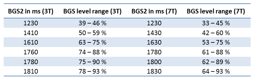
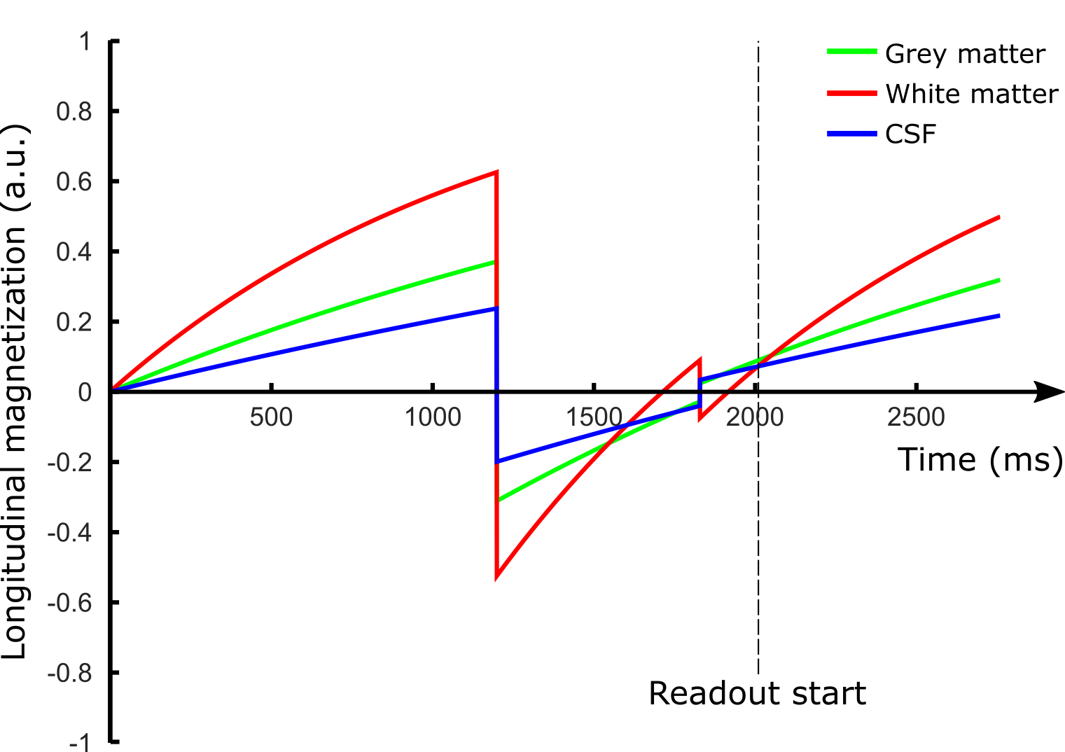
Background suppression-From a situation where the simulated BGS-level of grey-matter (GM), white-matter (WM) and cerebrospinal-fluid (CSF) was higher than 90% (Fig.1), the timings of the second BGS-pulse (BGS2) were changed to achieve six BGS-levels (Table 1). A BGS-level of 100% implies complete BGS and thus no signal of the static tissue. A non-BGS scan was acquired for comparison. The scans were acquired in random order.

Readout-Acquisition consisted of a multi-slice, single-shot EPI (resolution:3×3mm², 13 slices of 3mm, TI=2s, TR=4500ms). The inter-slice duration was 35ms at 3T and 64ms at 7T, yielding a different BGS-level for each slice, which was exploited to increase the number of studied BGS-levels.

A multi-TI FAIR was acquired to evaluate the tissue T₁, the equilibrium magnetization M₀ and the inversion efficiency of the FOCI-pulse. This scan was performed without pre-, post-sat and BGS.

Post-processing-Perfusion-weighted maps were calculated as the difference between the selective and the non-selective images. From the mean perfusion images over all scans a GM-mask was created. This GM-mask was applied to all image series.

The BGS-level was calculated for each slice of the non-selective images, as the relative difference with the M₀. The perfusion-tSNR was calculated voxel-wise as the signal-average over time divided by the standard-deviation over time. The obtained tSNR-values were normalized to those of the non-BGS-scan.

Statistics-To test whether the slopes of the curves in Fig.4 differed significantly, the Real Statistics Resource Pack software⁵ was used.

Results & Discussion

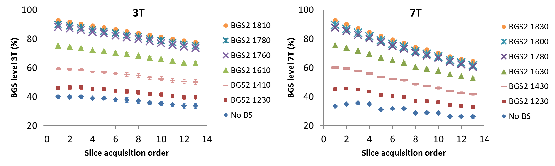
The BGS-level decreased with the slice number (Fig.2), reflecting that the static-tissue magnetization had more time to regrow for later-acquired slices. The BGS-level drop is stronger at 7T than at 3T, which can be explained by the difference in inter-slice time.

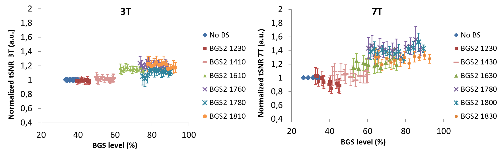
Fig.3 shows the normalized perfusion-tSNR across BGS-levels. At 7T, and in a lower extent at 3T, when BGS-pulses are introduced with timings generating low BGS-levels (e.g.BGS2=1230ms), the perfusion-tSNR deteriorates slightly. Such early BGS-pulses have indeed almost no effect on the static signal at the image acquisition time-point, but their non-perfect inversion destroys part of the ASL-signal, explaining the observed decrease⁶. The gain in perfusion-tSNR increases until BGS-levels around 70% after which a plateau is reached.

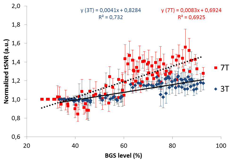
High BGS-levels (>80%) increase the perfusion-tSNR by 18% at 3T and 38% at 7T, in average, compared to a scan without BGS. Moreover, Fig.4 shows that the slope of the tSNR-increase as a function of BGS-level is twice as large at 7T as compared to 3T (p<0.01). It can therefore be concluded that suppressing the background-signal is much more important at higher magnetic field-strength.

BGS is known to be optimal for a 3D-readout that consists of a single excitation pulse per repetition time (TR)¹, because all slices will have the highest BGS-level. However, at high-field, high-quality fast 3D-images are harder to achieve, and a 2D-multislice readout might therefore be more appropriate. Our data show that a BGS-level higher than 70% is sufficient to improve the perfusion-tSNR. This gives a broader range of possible BGS-levels that will improve the perfusion-tSNR, and justifies the use of BGS in a 2D-multislice-readout. However, for the last-acquired slices in this study, the BGS-level was lower than 70%, and thus not optimal. Multiband is a logical candidate to shorten the readout time, just as strategies to achieve high BGS over multiple 2D-slices⁷.

Acknowledgements

References

1. Alsop, D. C. et al. Recommended implementation of arterial spin-labeled Perfusion mri for clinical applications: A consensus of the ISMRM Perfusion Study group and the European consortium for ASL in dementia. Magn. Reson. Med. 73, 102–116 (2015).

2. Dixon, W. T., Sardashti, M., Castillo, M. & Stomp, G. P. Multiple inversion recovery reduces static tissue signal in angiograms. Magn. Reson. Med. 18, 257–268 (1991).

3. Ye, F. Q., Frank, J. A., Weinberger, D. R. & McLaughlin, A. C. Noise reduction in 3D perfusion imaging by attenuating the static signal in arterial spin tagging (ASSIST). Magn. Reson. Med. 44, 92–100 (2000).

4. Reynaud, O., Jorge, J., Gruetter, R., Marques, J. P. & van der Zwaag, W. Influence of physiological noise on accelerated 2D and 3D resting state functional MRI data at 7 T. Magn. Reson. Med. 78, 888–896 (2017).

5. Charles Zaiontz. Real Statistics Resource Pack software. (2017).

6. Garcia, D. M., Duhamel, G. & Alsop, D. C. Efficiency of inversion pulses for background suppressed arterial spin labeling. Magn Reson Med 54, 366–372 (2005).

7. Shao, X., Wang, Y., Moeller, S. & Wang, D. J. J. A constrained slice-dependent background suppression scheme for simultaneous multislice pseudo-continuous arterial spin labeling. Magnetic Resonance in Medicine (2017). doi:10.1002/mrm.26643