2093
How does the weighting factor in a regularized quantitative BOLD approach affect the estimated oxygen extraction fraction?1Computer Assisted Clinical Medicine, Medical Faculty Mannheim, Heidelberg University, Mannheim, Germany
Synopsis
Applying the quantitative blood-oxygenation-level-dependent (qBOLD) method for measuring the oxygen extraction fraction (OEF) often suffers from bad contrast due to the low SNR typical at clinical scan times. In order to improve the evaluation, the choice of the weighting factors in a proposed regularization approach was analyzed. Using the regularization approach, simulations showed increasing precision but decreasing accuracy for increasing weighting factors. For a range of weighting factors a good trade-off between noise suppression and data-fidelity was achieved, which resulted in optimal contrast.
Introduction
The oxygen extraction fraction (OEF) in the brain can be measured by means of magnetic resonance imaging (MRI) on the basis of the blood-oxygenation-level-dependent (BOLD) effect and the tissue model proposed by Yablonskiy and Haacke.1 In order to improve the robustness of this quantitative BOLD2 method especially when applied to data with low signal-to-noise-ratio (SNR),3 a regularization approach has recently been proposed, which stabilizes the least-squares (LS) regression by penalizing deviations from prior information.4 In regularization the choice of the weighting parameter plays an important role. Therefore, this work systematically analyzes the effect of the weighting factor on the OEF contrast in a simulation to determine the parameter settings yielding an optimal contrast.Methods
A 128x128 pixels OEF map was created with the upper half set to a baseline value of 40%, typical for the healthy human brain.5 An increased OEF of 80% was assigned to the lower half of the map representing a hotspot of high oxygen demand. To simulate the MR signal magnitude corresponding to a gradient-echo-sampled-spin-echo (GESSE) sequence, the following model was assumed1:
$$ \ln\left(\frac{S(t)}{S_{SE}}\right) = -\frac{1}{3}\int_{0}^{1} (2+u)\sqrt{1-u} \cdot \lambda \frac{1-J_{0}(a\cdot \text{OEF} \cdot u \cdot t)}{u^{2}} \text{d}u - R_2 t $$
Standard parameters (SSE=100, R2=12Hz, λ=2%)2 and the OEF map were used to simulate the signal for N=32 echo times. Gaussian noise with a standard deviation typical for the in-vivo case was added (SNR=80). In order to reversely calculate the OEF map using regularized regression, the following cost-function was defined4:
$$ \underset{S_{SE},R_2,OEF,\lambda}{\mathrm{argmin}} \left\{ \sum_{n=1}^N [y_n - S(\text{TE}_{n})]^2 + w (\text{OEF}-\text{OEF}_{prior})^2 + c \cdot w (\lambda - \lambda_{prior})^2 \right\} $$
OEFprior and λprior were set to 40% and 2% respectively. The regularization terms were controlled by the weighting factor w, which was varied from 10-3 to 103. The last term was scaled by the factor c to account for different magnitudes of the regularization terms.
Results
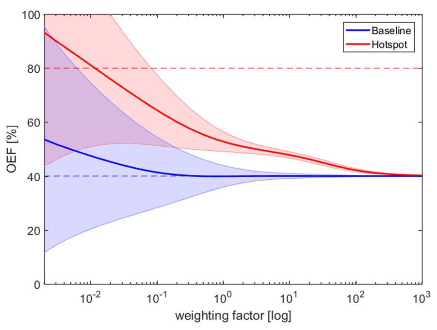
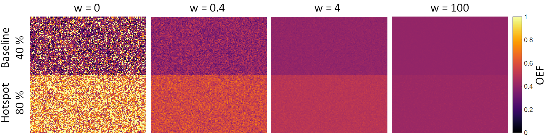
As depicted in Figure 1, the mean values and standard deviations of the baseline and hotspot region are reduced from (54 ± 42)% to (40 ± 0.02)% and (93 ± 50)% to (40 ± 0.04)% respectively with increasing weighting factor. Since both regions converge towards the prior, an increasing bias is introduced with rising weighting factor especially in the hotspot region. As the variances of both regions concurrently decrease, a range of weighting factors from approximately 0.2 to 200 is observable, in which the mean values do not overlap within one standard deviation. OEF maps with exemplary weighting factors (0; 0.4; 4; 100) are shown in Figure 2. While the OEF contrast is corrupted by noise for the LS regression (w=0) and almost completely smoothed out in the case of a very high weighting, a balanced contrast is visible for moderate weighting factors.Discussion
In contrast to the noise dominated LS regression, the regularization approach suppresses the influence of noise on the estimated OEF. Therefore, the precision of the estimates increases with the weighting. Due to the penalty for solutions that deviate from the prior, hotspots experience a bias from their true value, which leads to a decreased accuracy for higher weightings. For moderate weighting, a trade-off between noise-suppression and data-fidelity leads to a distinct contrast between hotspot and baseline and thus to an advantage of the regularization approach over conventional LS regression. Remarkably, the range of this enhanced contrast spans over approximately three orders of magnitude, which makes it robust against an imperfect choice of weighting.Conclusion
The influence of different weighting factors of the regularization term on the estimated OEF was analyzed for a map comprising a baseline level (40%) and a region of increased OEF (80%). The simulations show an increasing suppression of the otherwise dominating noise for higher weighting and a broad range of weighting factors was found facilitating improved discrimination of baseline and hotspot. This ability to distinguish hotspots from baseline OEF yields a major advantage compared to conventional LS regression.Acknowledgements
The authors thank the Deutsche Forschungsgemeinschaft for their financial support within the framework of the “Nachwuchsakademie Medizintechnik” (reference number: DO 1955/1-1).References
1. Yablonskiy DA, Haacke EM. Theory of NMR signal behavior in magnetically inhomogeneous tissues: the static dephasing regime. Magn Reson Med. 1994. 32(6):749-63.
2. He X, Yablonskiy DA. Quantitative BOLD: mapping of human cerebral deoxygenated blood volume and oxygen extraction fraction: default state. Magn Reson Med. 2007. 57(1):115-26.
3. Sedlacik J, Reichenbach JR. Validation of quantitative estimation of tissue oxygen extraction fraction and deoxygenated blood volume fraction in phantom and in vivo experiments by using MRI. Magn Reson Med. 2010. 63(4):910-21.
4. Domsch S, Weingärtner S, Zapp J, et al. Regularized least-squares regression analysis for quantitative BOLD. Magn Reson Mater Phy. 2015. 28(1):158.
5. Gusnard DA, Raichle ME. Searching for a Baseline: Functional Imaging and the Resting Human Brain. Nature. 2001. 2(October):685-694.
Figures