1870
Vector Field Perfusion Imaging: A Validation Study by Using Multiphysics Model1Department of Radiology, Weill Cornell Medical College, New York, NY, United States, 2Institut de Mécanique des Fluides de Toulouse, Toulouse, France, 3Department of Biomedical Engineering, Cornell University, Ithaca, NY, United States
Synopsis
A multiphysics model based on Navier-Stokes equation and continuity equation is built to simulate the arterial spin labeled (ASL) blood flow in the blood vessels. Blood velocity distribution is reconstructed by measuring the 4D time-resolved labeled blood concentration and doing inversion data fitting processing. The conventional lumped-element Kety’s equation provides a quantitative measurement of whole brain cerebral blood flow (CBF) suffering from the inaccurate estimation of arterial input function (AIF). The multiphysics model validates that the blood velocity involved vector field perfusion (VFP) with multiple post label delays does not rely on the AIF.
Introduction
Perfusion imaging, indicating the blood flow at small vessels and capillaries, is of great importance for managing patients with a various disease, including stroke, heart attack, and cancel. Current quantification of perfusion is based on Kety’s equation, which requires the arterial input function (AIF) as an input1. However, AIF cannot be measured during imaging and is usually assumed to be same in the brain. This assumption ignores the tracer delay and dispersion, and causes large errors and poor reproducibility2. In this abstract, we validate the biophysically based vector field perfusion (VFP)3 by using multiphysics model in which AIF is not needed.Theory
The validation includes a forward multiphysics model to generate ground truth blood velocity and tracer concentration, and an inverse optimization model to reconstruct the velocity distribution from measured tracer concentration.
Forward model: The blood velocity$$$\,{\bf u}\,$$$in the vessel is governed by the Navier-Stokes equation and the incompressibility assumption
$$$\rho\frac{\partial{\bf\,u}}{\partial\,t}+\rho({\bf\,u}\cdot\nabla){\bf\,u}=\nabla\cdot[-p{\bf\,I}+\mu(\nabla{\bf\,u}+(\nabla{\bf\,u})^T)],\qquad\rho\nabla\cdot{\bf\,u}=0\qquad\qquad$$$[1]
with certain boundary conditions, where$$$\,\rho\,$$$is the density of the blood,$$$\,p\,$$$is the pressure, and$$$\,\mu\,$$$is the viscosity of blood. Given the velocity field$$$\,{\bf u}\,$$$computed from Eq. [1], then the tracer concentration$$$\,c\,$$$satisfies the continuity equation
$$$\frac{\partial\,c}{\partial\,t}=-\nabla\,c\cdot{\bf\,u}-\gamma\,c+\nabla\cdot(D\nabla\,c)\qquad\qquad$$$[2]
with boundary conditions, where$$$\,\gamma\,$$$is the signal decaying rate, $$$\,\gamma=1/T_1\,$$$for ASL , and$$$\,D\,$$$is the diffusion coefficient.
Inverse model: Given the 4D time-resolved concentration from [2], with the assumption that the velocity$$$\,{\bf\,u}=(u,v,w)^T\,$$$is time independent, it is remaining to recover the blood velocity by solving the following minimizing problem4 without the requirement of AIF
$$$\min_{\bf\,u}\sum_{k=1}^N\left[\left\|\frac{\partial\,c^k}{\partial\,t}+\nabla\,c^k\cdot{\bf\,u}+\gamma\,c^k-\nabla\cdot(D\nabla\,c^k)\right\|^2\right]+\alpha\left(\|\nabla\,u\|^2+\|\nabla\,v\|^2+\|\nabla\,w\|^2\right),\qquad\qquad$$$[3]
where$$$\,\|\cdot\|\,$$$is the standard Euclidean norm and$$$\,\alpha\,$$$is the regularization parameter as a trade-off between the data fitting term and regularization term for smoothness of the solution,$$$\,N\,$$$is the number of time points for data sampling.$$$\,D\,$$$is assumed to be zero since the diffusion effect is minor.
Methods
A numerical phantom of blood vessel structure is generated to demonstrate the velocity reconstruction by [3]. First, we numerically demonstrate that the solution of [3] is close to the ground truth when the concentration is sampled with high resolution, i.e., the voxel size is smaller than the vessel size. Second, we generated low-resolution data by averaging the high-resolution data to make voxel size larger than the vessel size. It shows that the vessel structure plays a critical role to the solution of [3] with low-resolution data and in this case, the velocity could be misestimated. Third, we tested the algorithm [3] with in vivo data from 8 healthy subjects to validate the reconstructed velocity distribution.Results
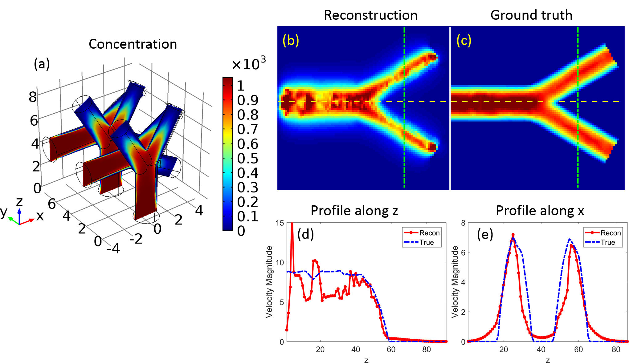
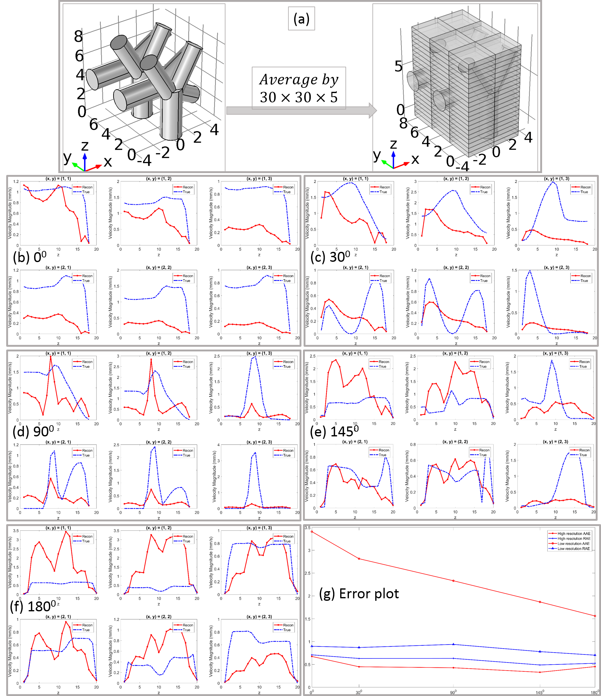
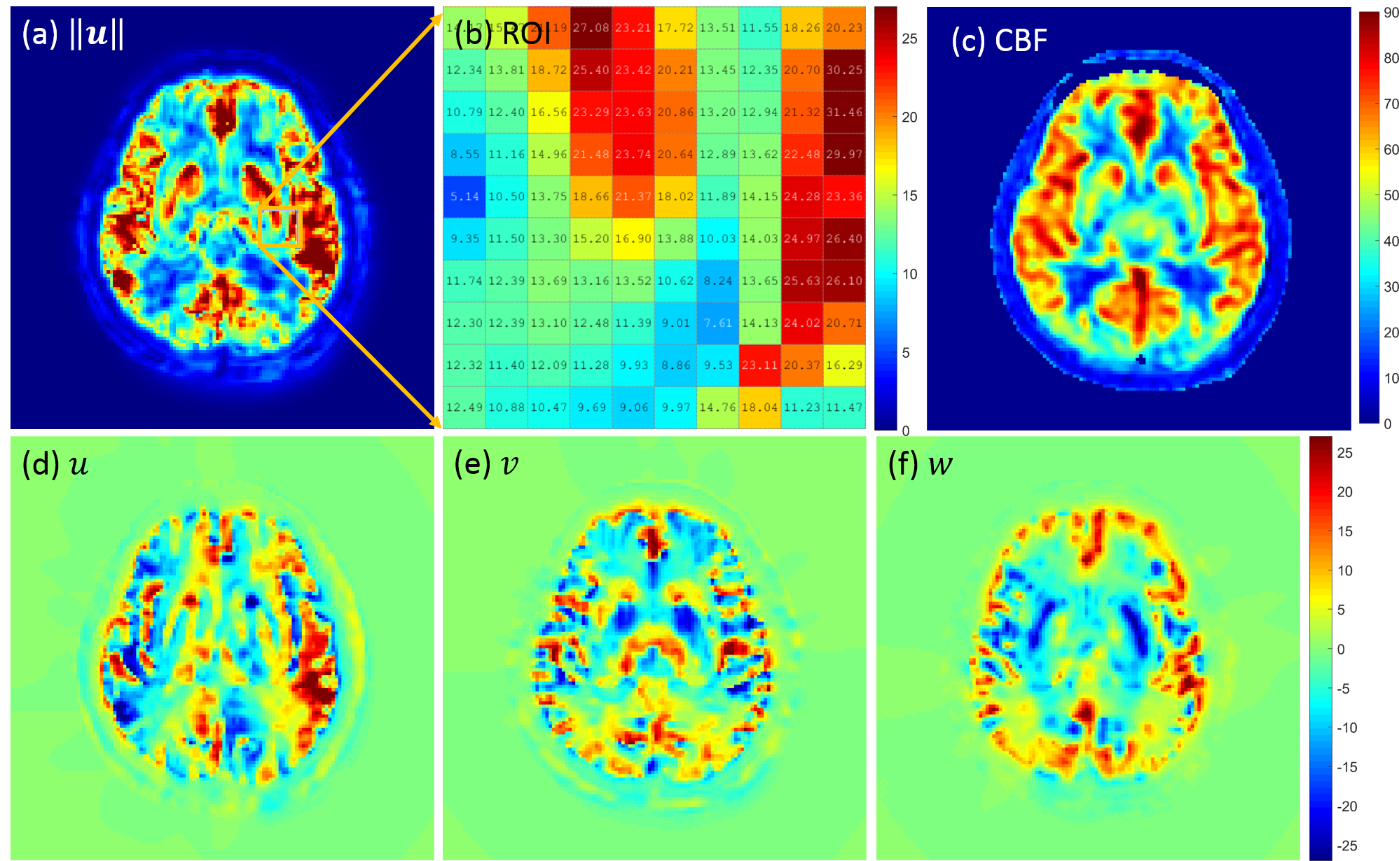
Fig.1 shows the numerical phantom design and the forward model solutions$$$\,{\bf\,u}\,$$$oand$$$\,p\,$$$of [1]. Fig. 2 shows the accurate velocity reconstruction by [3] with high-resolution data. Fig.3 shows the solution of [3] with averaged low-resolution data and their errors. The results imply that the velocity from [3] with low-resolution data is a weighted combination of the individual velocity of each branch of vessels. As the vessel structure gets more complex, the reconstructed velocity gets more overestimated. The reconstruction errors for all the 5 models are shown in Fig.3 (g). Fig.4 shows the results from in vivo human data. The overestimation rate may be determined by a calibration method.Discussion
Generally, MRI data is acquired at low resolution with voxel size larger than the vessel size. This leads to the partial volume effect and velocity superposition. The nonlinear relation between$$$\,c\,$$$and$$$\,{\bf\,u}\,$$$makes the sampled low-resolution data inconsistent with the superposed velocity. Assume$$$\,{\bf\,u}\,$$$is sufficiently smooth and$$$\,\alpha=0\,$$$in [3], then [3] becomes least square and its high-resolution solution for only one branch of blood vessel can be explicitly expressed as
$$${\bf\,u}_1=({\bf\,A}_1^T{\bf\,A}_1)^{-1}{\bf\,b}_1\quad\,\mbox{with}\,{\bf\,A_1}:=\begin{bmatrix}c_{1x}^1&c_{1y}^1&c_{1z}^1\\\vdots&\vdots&\vdots\\c_{1x}^N&c_{1y}^N&c_{1z}^N\end{bmatrix},\,{\bf\,b}_1:={\bf\,A}_1^T{\bf\,r}_1,\,{\bf\,r}_1=\begin{bmatrix}r_{11}\\\vdots\\r_{1N}\end{bmatrix},\,r_{1i}=-\frac{\partial\,c_1^i}{\partial\,t}-\gamma\,c_1^i+\nabla\cdot(D\nabla\,c_1^i),\qquad\qquad$$$[4]
where$$$\,c_1^i\,$$$denotes the concentration for the 1st branch at time point$$$\,i$$$, and$$$\,c_{1x}^i\,c_{1y}^i\,$$$and$$$\,c_{1z}^i\,$$$are the components of the gradient of$$$\,c_1^i$$$.
However, if there are more than one vessel branches (e.g.$$$\,M\,$$$branches) in the large voxel region, the measured data is the total concentration of all the branches. Then the solution of [3] at low-resolution is represented as
$$${\bf\,u}_{1M}=\left(\mathbb{A}_M^T\,\mathbb{A}_M\right)^{-1}{\bf\,b}_{1M},\,\mbox{with}\,{\bf\,b}_{1M}:=\mathbb{A}_M^T\,{\bf\,R}_M\qquad\qquad$$$[5]
where $$$\mathbb{A}_M:={\bf\,A}_1+\cdots+{\bf\,A}_m+\cdots+{\bf\,A}_M$$$ and $$${\bf\,R}_M={\bf\,r}_1+\cdots+{\bf\,r}_m+\cdots+{\bf\,r}_M,$$$
and $$$\,{\bf\,A}_m\,$$$and$$$\,{\bf\,r}_m\,$$$ for all $$$m=1,\cdots,M$$$ are defined in the same way as$$$\,{\bf\,A}_1\,$$$and$$$\,{\bf\,r}_1\,$$$in [4], respectively. It is clear to see that$$$\,{\bf\,u}_{1M}\,$$$in [5] is a weighted combination of$$$\,{\bf\,u}_1\,$$$to$$$\,{\bf\,u}_M$$$, and other terms related to the interaction between$$$\,M\,$$$branches. This can also be seen in the simulated results in Fig.3 and the errors in Fig.4, as well as the in vivo results in Fig.5.
Conclusion
We validated the solution of VFP by using multiphysics model. The velocity recovered in VFP of the large voxel is concentration gradient driven, a weighted combination of velocity in all the vessel branches located in the voxel. This is useful for further calibration of the accuracy of the vector field perfusion algorithm. The CBF can then be calculated from$$$\,{\bf\,u}\,$$$in [3].Acknowledgements
No acknowledgement found.References
[1] Kety SS. The Theory and Application of the exchange of inert gas at the lungs and tissues. Pharmacol. Rev. 3(1):1-41, 1951. [2] Calamante F. Arterial Input Function in Perfusion MRI: A Comprehensive Review. Prog. Nucl. Mag. Reson. Spectrosc. 74:1-32, 2013. [3] Spincemaille P, Zhang Q, Nguyen TD, Wang Y. Vector Field Perfusion Imaging. Proc. Intl. Soc. Mag. Recon. Med. 25, 2017. [4] Horn BKP, Schunck BG. Determining Optical Flow. Artif. Intl. 17(1-3):185-203, 1981.Figures
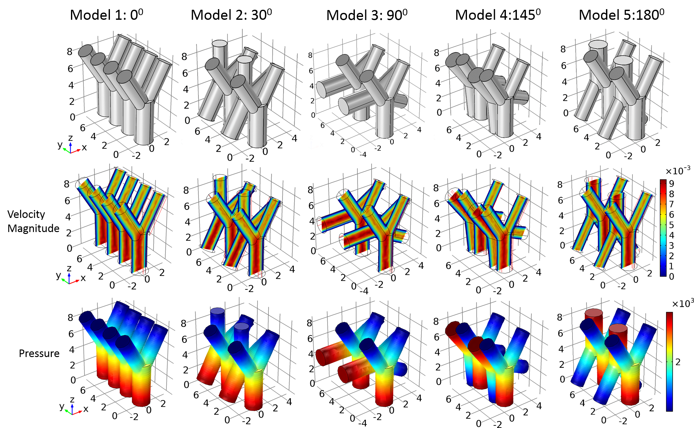
- Fig.1 Numerical phantom design and solutions of [1]. The first row shows the blood vessel models, each with four simple bifurcation blood vessels of different rotation angles. The diameter of the inlet/outlet tube is 2mm/1.6mm. From left to right, the rotation angles of two bifurcation blood vessels are 00, 300, 900, 1450 and 1800, respectively. The second and third rows show the solutions$$$\,{\bf\,u}\,$$$and$$$\,p\,$$$of [1] for each model. The units for this abstract are: length (mm), velocity (mm/s), pressure (Pa), concentration (kg/m3), time (s).