1857
Myelin-Water Quantification: Orthogonal Matching Pursuit versus Non-Negative Least Squares1Department of Radiology & Nuclear Medicine, Maastricht University Medical Center, Maastricht, Netherlands, 2School for Mental Health and Neuroscience, Maastricht University Medical Center, Maastricht, Netherlands, 3Department of Behavioral Sciences, Epilepsy Center Kempenheaghe, Heeze, Netherlands
Synopsis
Myelin-water quantification relies on modeling of multi-exponential T2-relaxation time decay. For this, we explore the greedy Orthogonal Matching Pursuit (OMP) method and compare it to the most commonly applied non-negative least squares (NNLS) method. The two methods are evaluated by means of simulations, phantom measurements and in vivo image data.
Purpose
Multi-Spin-Echo (MSE) pulse sequences can yield in vivo estimates of myelin-water content by splitting the multi-exponential T2 relaxation signal into its constituting components. This multi-component analysis is most commonly performed using a regularized version of the non-negative least squares (NNLS) method, which extends on bi-exponential curve fitting by making no assumptions on the number of components and not requiring a starting model1. Using a basis set of relaxation functions (i.e. dictionary) the NNLS method estimates the corresponding amplitudes. However, due to its computational complexity it is restricted to a relatively low resolution dictionary, furthermore, it has a large amount of unknown parameters and thus needs strong regularization. In the current study we explore whether the Orthogonal Matching Pursuit (OMP) can be used as an alternative method for identifying the underlying components. Simulations, phantom measurements and in vivo data are used to validate the multi-component analysis.Methods
The greedy OMP algorithm builds a sparse representation of the signal by iteratively selecting that particular element from a dictionary which correlates most with the current residual2. Therefore, similarly to NNLS, no starting model is needed. Non-negativity is guaranteed for each iteration by solving a non-negative least squares problem for the current selection of elements2. To increase the stability of the algorithm, it is called 20 times per voxel (the OMP is roughly 20 times faster than NNLS).
To estimate the theoretical errors of the NNLS and OMP algorithms, relaxation data were synthesized using the extended phase graph (EPG)3 algorithm (flip angle 150⁰). The relaxation times were chosen to match those of the in vivo content (T1=860ms, T2long=88ms, and T2myelin=30ms). For simulations, noise was estimated from the in vivo image acquisition. To assess the effects of myelin content on the analysis, 1000 Gaussian noise realizations were performed for a varying myelin-water content (range 0-30%).
To estimate errors in MWF estimation due to the MSE sequence, two mono-exponential manganese(II)-chloride vials were constructed with T2 values of 30 and 110ms. Multi-exponential decays were synthesized by summing two randomly chosen voxels from each phantom and weighing them such that a varying MWF (range 0-30%) was obtained. This process was repeated 1000 times.
To visualize the difference of the two methods in vivo, three healthy male volunteers were scanned (aged 28-30). The vials and volunteers were scanned on a 3.0T unit (Philips Achieva) using a single-slice MSE sequence4 (TR=3000ms, TE=12ms, 32 echoes, voxel size 1.5x1.5x4 mm, 2 signal averages). The EPG algorithm was used to correct for B1-inhomogeneities.
Lastly, a dictionary with 120 and 1000 logarithmically spaced T2 values between 10 and 3500ms was used for the NNLS and OMP, respectively.
Results
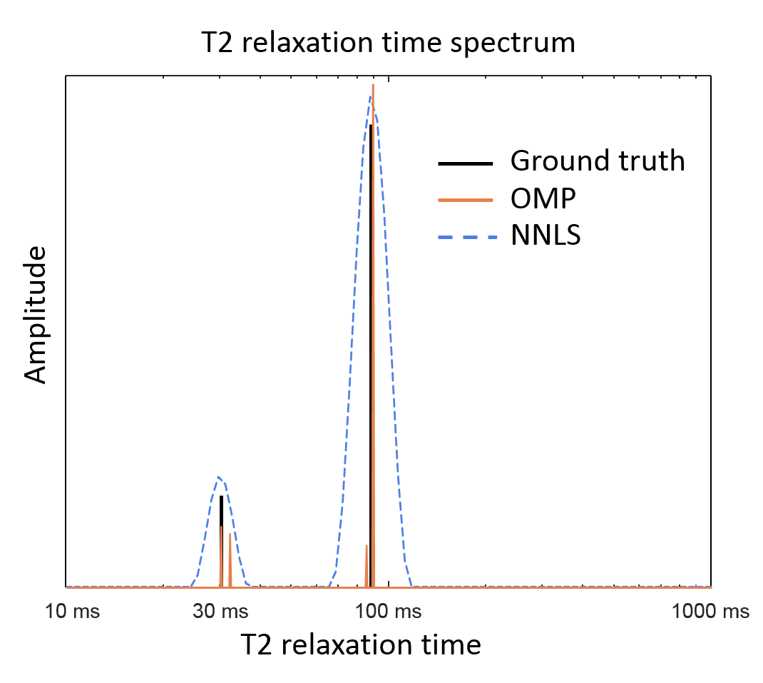
In Figure 1 an example solution is shown to visualize the difference between the NNLS and OMP output spectra. In this example a noisy signal comprising of two components (at 30 and 88ms) and a MWF of 15% is solved by both methods.
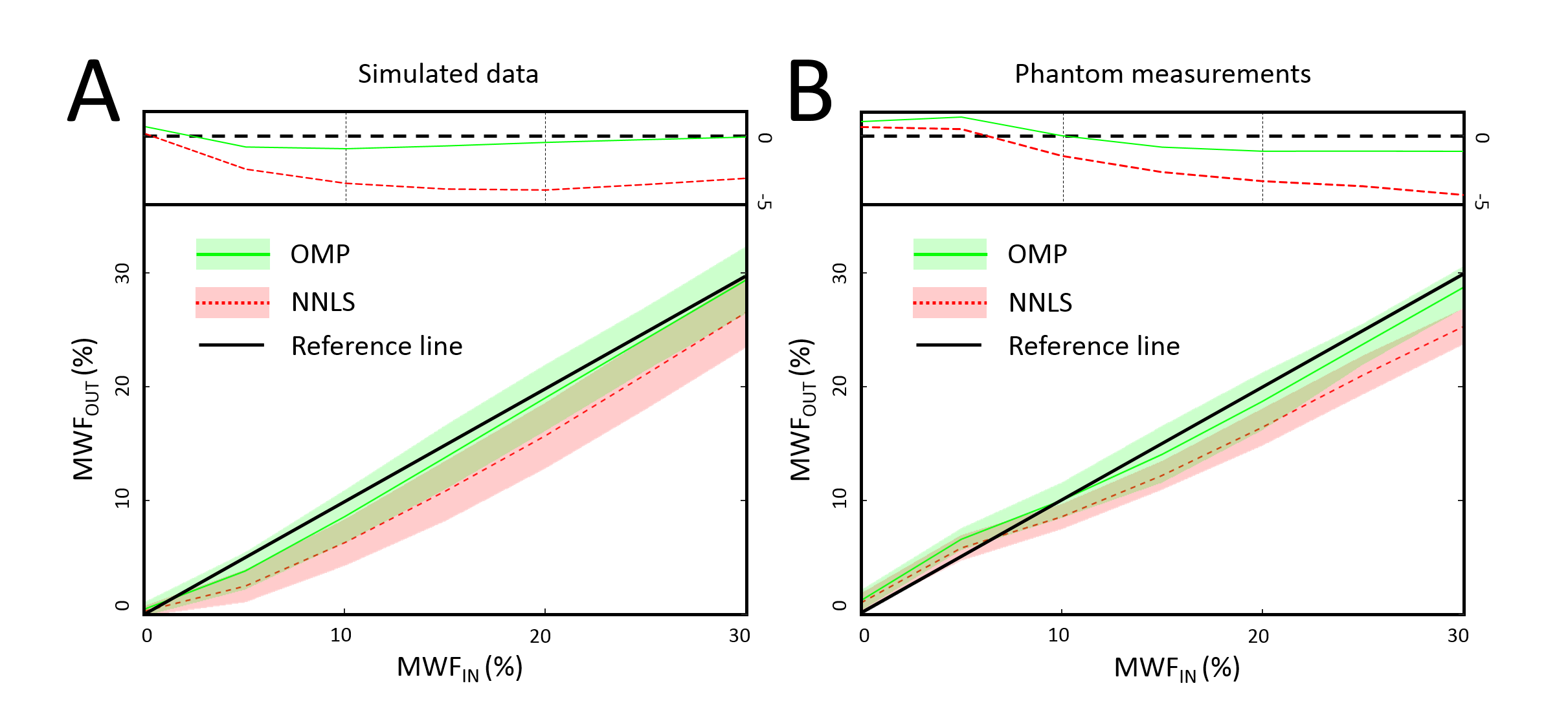
In Figure 2 the results of the simulations and phantom measurements are shown. For a specific MWF of 15% the analysis of the simulated data results in an underestimated mean MWF of 13.8% (OMP) and 11.8% (NNLS), for the phantom measurements the estimated MWF is 14% (OMP) and 12.2% (NNLS). Therefore, the OMP is approximately 3.5 times ($$$\left|\frac{15\%-\mu_{NNLS}}{15\%-\mu_{OMP}}\right|$$$) closer to the true mean compared to NNLS for the simulated data, and approximately 3 times for the phantom measurements. Both methods show a similar precision (variation on the mean).
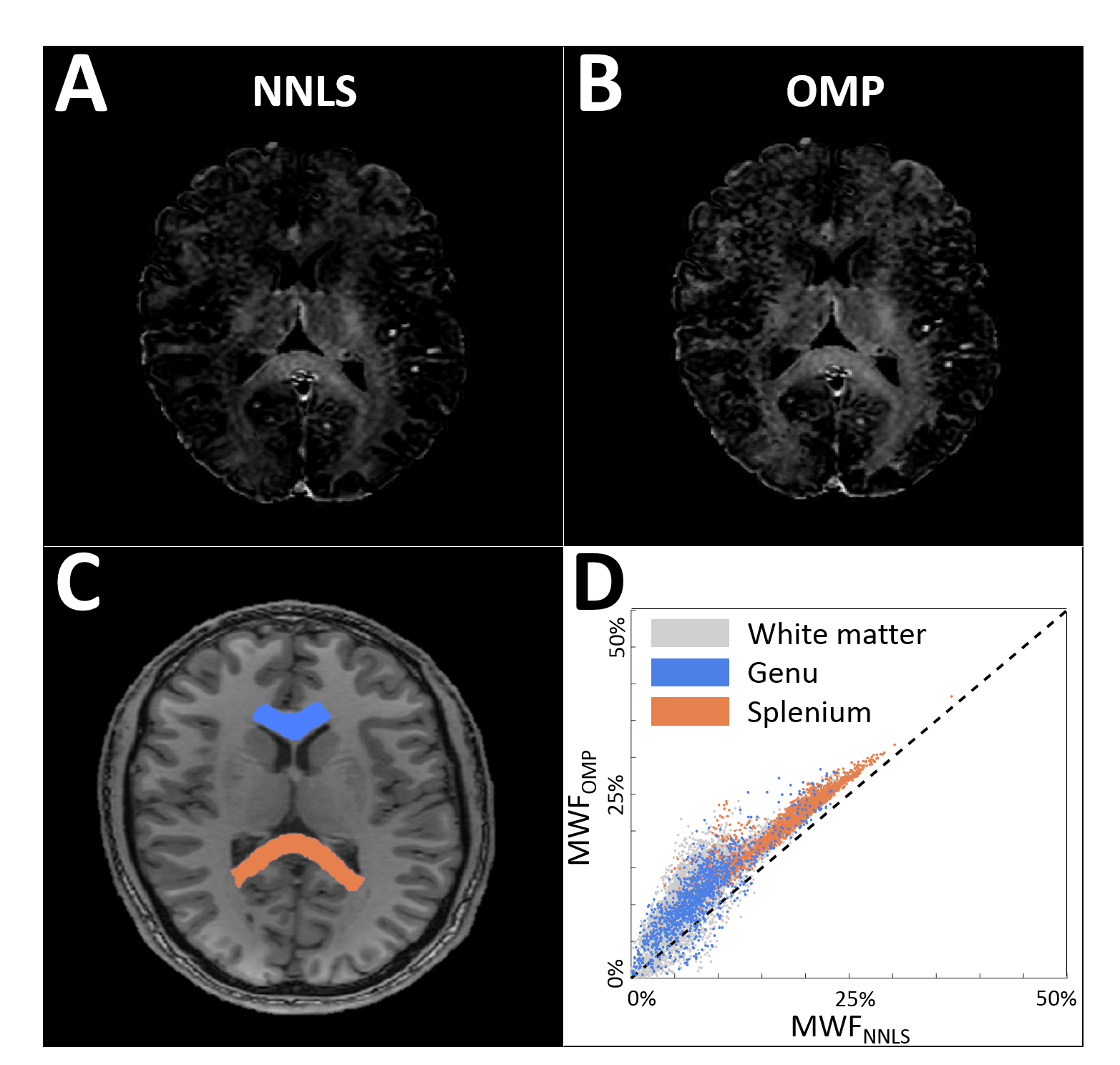
The MWF map of a healthy volunteer is shown in Figure 3. As region of interests, the splenium and the genu of the corpus callosum were delineated in the white matter. In each region the MWFs obtained with the OMP were, on average, higher in comparison to the NNLS (splenium: 21.1%±4.4% vs 17.7%±4.9% and genu: 11.3%±5.1% vs 8.0%±4.3%). These MWF values agree well to those reported in previous studies5.
Discussion & Conclusion
OMP is an approximately 3 times more accurate measure for MWF quantification compared to NNLS. Most likely this is due to the increased resolution of the T2 relaxation time spectrum (e.g. larger dictionary). The simulations and phantom measurements show that both the NNLS and OMP tend to underestimate the true MWF. Possibly the underestimation occurs when part of the amplitude peak has a too short T2 value, which is compensated by a higher amplitude. This effect is stronger for higher T2 values where the resolution is lower due to the logarithmic spacing. Therefore, the OMP, having a higher resolution dictionary, is less prone than NNLS to the MWF underestimation and therefore more accurate for myelin-water quantification.
Acknowledgements
No acknowledgement found.References
1. Whittall K. Quantitative interpretation of NMR relaxation data. J Magn Reson. 1989;84:134-152.
2. Yaghoobi M, Wu D, Davies M. Fast Non-negative orthogonal matching pursuit. IEEE Signal Processing Letters. 2015;22(9):1229-1233.
3. Hennig J. Multiecho imaging sequences with low refocusing flip angles. J Magn Reson. 1988;78:397–407.
4. Kolind S, Madler B, Fisher S, et al. Myelin water imaging: implementation and development at 3.0T and comparison to 1.5T measurements. Magn Reson Med. 2009;62:106-115.
5. Prasloski T, Madler B, Ziang Q, et al. Applications of stimulated echo correction to multicomponent T2 analysis. Magn Reson Med. 2012;67:1803-1814.
Figures