1773
Evaluation of cortical thickness estimation methods in neonates.1Medical Physics Department, IRCCS Bambino Gesù Children’s Hospital, Rome, Italy, 2Enginerring Department, Roma Tre University, Rome, Italy, 3Imaging Department, IRCCS Bambino Gesù Children’s Hospital, Rome, Italy
Synopsis
Cortical thickness (CT) is a sensitive indicator of normal brain structural and functional development, aging, as well as a variety of neuropsychiatric disorders. The state of the art for cortical thickness estimation in children in not as good as the one for adults. We then compared two different algorithms and assess the agreement between these methods and their local variability.
Introduction
Cortical thickness (CT) is a sensitive indicator of normal brain structural and functional development, aging, as well as a variety of neuropsychiatric disorders (1). These considerations generated an increasing interest for the early development of CT, resulting in several recent studies aiming to investigate it from birth until the second postnatal year (2). An accurate CT estimation relied on MR images segmentation procedures, but although algorithms exist for adult subjects, most of them cannot be extended to infant brain due to the low tissue contrast and high within-tissue intensity variability of images. Despite FreeSurfer (FS) is one of the major software packages for MR images elaboration, it guarantees accurate segmentation only for adult subjects. Conversely, Computation Anatomy Toolbox (CAT), a novel SPM-based tool developed at Jena University is able to segment and compute CT in adult and infant data (3). The CAT’s CT computation makes use of a projection-based thickness (PBT) algorithm that exploits tissue segmentation to compute white matter (WM) distance, then projects local maxima (equal to the CT) to the grey matter (GM) voxels and finds thickness distribution using neighbour relationship described by WM distance itself (3). On the other hand, FS based the estimate of CT on the difference between inner and outer cortical surface with a nearest neighbour correspondence (4). The aim of this study is then to evaluate infant CT estimation goodness for both methods in order to improve the understanding of CT developing during infancy.Methods
We acquired 3D T2 weighted Turbo Spin Echo sequences on a 3T Siemens Magnetom Skyra scanner of 12 healthy subjects (mean age = 16 weeks) recruited at the Pediatric Hospital Bambino Gesù (Rome). CAT segmentation pipeline performs correction, registration and global/local intensity normalization of the input data, producing skull-stripped volumes segmented into GM, WM and cerebro-spinal fluid. After segmentation CAT measures CT with PBT algorithm, a method that handles the partial volume effects (PVE), sulcal blurring and asymmetries. Starting from CAT segmented volume we also use FS for CT estimation (Surface-based approach: SBA). To this purpose, we create an ad hoc MATLAB script able to combine the codes recalling part of the recon-all FS pipeline for CT estimation. For statistical purposes and visualization, we used an infant surface template available on UCN website (5). Average thickness values across regions are computed using UCN parcellation atlas information (5). We first assess correlation between average CT values from CAT and FS over the entire surface and then we limit the analysis to those regions that are not critical for the estimation algorithm. Local thickness variability map is computed by considering for each surface vertex a small region of neighbourhood points and calculating the variation coefficient within this area. Values are computed over the entire surface and then evaluated in each single label.Results
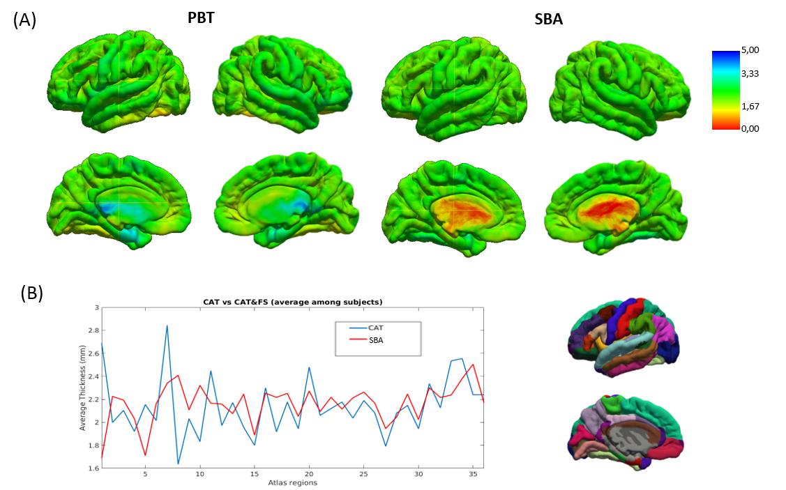
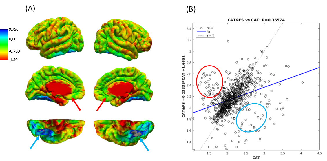
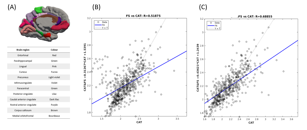
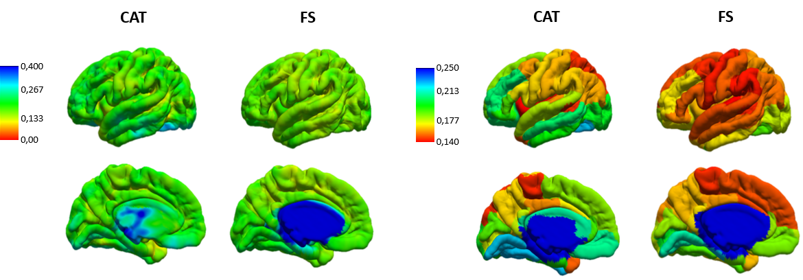
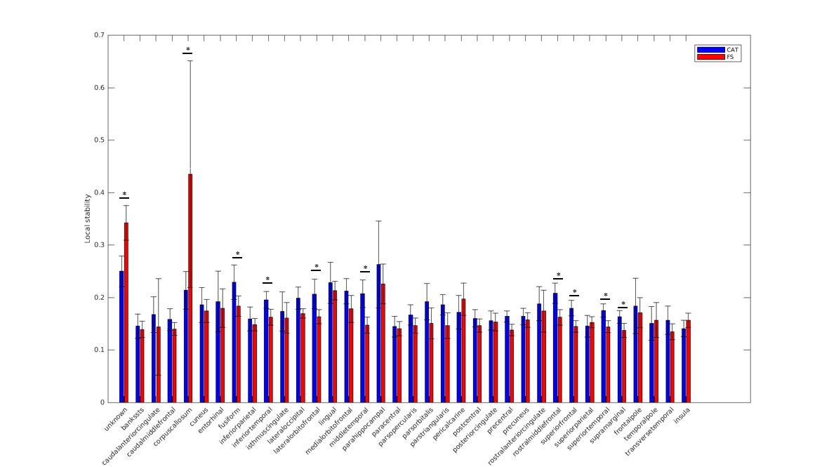
After mapping CT values on an infant surface template for both methods (Fig 1A), we obtained averaged CT distribution over 36 brain regions showing similar trend for CAT and FS (Fig 1B). Similar thickness was found for FS (2.16±0.17 mm) and CAT (2.14±0.26 mm). Mean difference map (Fig 2A) highlights the labels in which the algorithms differ most. Correlation between CT averaged in each brain areas and for each patient for CAT and FS shows very low R-value(Fig 2B), mainly due to the difficulty in estimating CT in specific regions close to the midline. When the analysis is not extended to the midline-close labels (Fig3A) we note a better correlation value (Fig3B) that is further improved excluding labels (fusiform and inferior temporal) where CAT over- and underestimates thickness compared to FS(Fig3C). Local thickness variability map for CAT and FS is measured in term of vertex-wise (left) and region-wise (right) variation coefficient (Fig4). Moreover, we quantify local thickness variability across labels measuring variation coefficient for each region from both CAT and FS (Fig4). FS variation coefficient has values similar to CAT for almost regions, but there is statistically significant differences in few brain areas (Fig5).
Discussion
We evaluate CAT and FS as tool for infant CT estimation. Results suggest similar thickness distribution except for specific regions (brain midline) where estimation is critical and mostly depends on the different approaches used for CT estimation. Evaluation of local stability suggests slightly better results for FS approach that consequently could represent a valid option as thickness estimation tools for infants.Conclusion
Evaluating CT estimation methods for infant subjects could represent a step towards a better understating of cortex development, allowing early diagnosis of several neurological diseases. Both algorithms are valid tool for estimating the thickness in adults but there is still an ongoing work to do on the assessment of these tools in neonates.Acknowledgements
No acknowledgement found.References
[1] Meng Y, Li G, Rekik I, Zhang H, Gao Y, Lin W, Carolina N (2017). Can we predict subject-specific dynamic cortical thickness maps during infancy from birth? Human Brain Mapping
[2] Li G, Lin W, Gilmore JH, Shen D (2015a): Spatial Patterns, Longitudinal Development, and Hemispheric Asymmetries of Cortical Thickness in Infants from Birth to 2 Years of Age.J Neurosci 35:9150–9162.
[3] Dahnke R, Yotter RA, Gaser C (2013): Cortical thickness and central surface estimation. NeuroImage; 65:336-48
[4] Dale AM, Fischl B, Sereno MI (1999): Cortical surface-based analysis. I. Segmentation and surface reconstruction. NeuroImage; 9(2):179-94
[5] Li G, Wang L, Shi F, Gilmore JH, Lin W, Shen D (2015b):Construction of 4D high-definition cortical surface atlases of infants: Methods and applications. Med Image Anal 25:22–36.
Figures