1762
Optimization of a traversable wire path of a gradient coil for a magnetic resonance microscope1Human Health Sciences, Graduate School of Medicine, Kyoto University, Kyoto, Japan, 2Center for the Promotion of Interdisciplinary Education and Resarch, Kyoto University, Kyoto, Japan
Synopsis
We designed 1 T/m gradient coils for a 14.1 T magnetic resonance microscope. The calculated contour wire pattern, however, should be transformed to a traversable wire path for actual construction. In this study, we optimized a connecting method by comparing three loop connecting patterns with the inside and outside return paths as a function of the transition size. We found that larger transition size in smooth parts of the loop reduced more the root mean square of deviations from the center gradient value. This optimization is applicable to gradient coils of larger size.
Introduction
MR microscopy requires higher magnetic field and stronger gradient field to achieve higher spatial resolution. We designed gradient coils for a 14.1 T magnet with a 48 mm bore that would produce 1 T/m gradient field in 20 mm × 20 mm × 30 mm ellipsoidal imaging volume by using a boundary element method.1 Calculated wire paths of the gradient coils from the stream-function, however, gives us only contour wiring patterns. In this study, we optimized a traversable wire path to have higher gradient field uniformity.Method
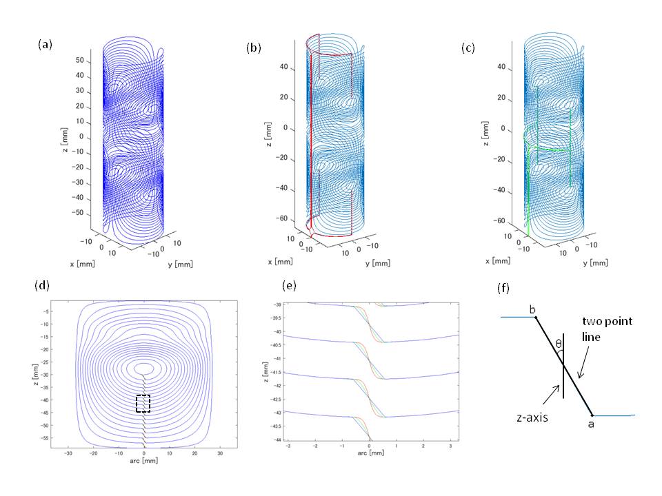
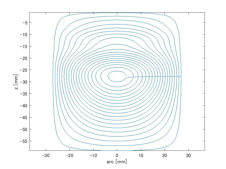
We designed a wire path of the x-axis gradient that would generate 1 T/m at 40 A within 300 μsec in the imaging volume and be located at most inner shell (ID 34 mm, OD 36 mm, length 120 mm) of our gradient system (Fig. 1 (a)). We compared the ideal wire path with two actual wire paths including the outside (Fig. 1 (b)) and inside (Fig. 1 (c)) return paths. We also compared three loop connecting patterns (Fig. 1 (d, e)): hyperbolic tangent (red), sine (green), straight line (blue). The three connecting patterns shared the same loop endpoints (Fig. 1 (f) a, b) that were defined as cross points with loops of a line making the predetermined angle to the z-axis. To evaluate characteristics of the gradient field uniformity, we calculated magnetic field at mesh points of 1 mm × 1 mm × 1 mm and extracted nonuniformity, variance, root mean square as follows:
$$$Nonuniformity=\frac{1}{V}\int_{}^{}\frac{\mid G(r)-G_{0} \mid}{G_{0}}\times100\,dr\\Root\ Mean\ Square=\sqrt{\frac{1}{V}\int_{}^{}\left(\frac{G(r)-G_{0}}{G_{0}}\times100\right)^{2}dr }$$$
where V, G(r), G0 are the imaging volume, gradient values at point r and the center, respectively. The variance was taken in the mesh points in the imaging volume. Moreover, we compared changes of the three characteristics due to difference of the connecting patterns. In this study, we optimized only the x-axis gradient which condition was constrained most.
Result
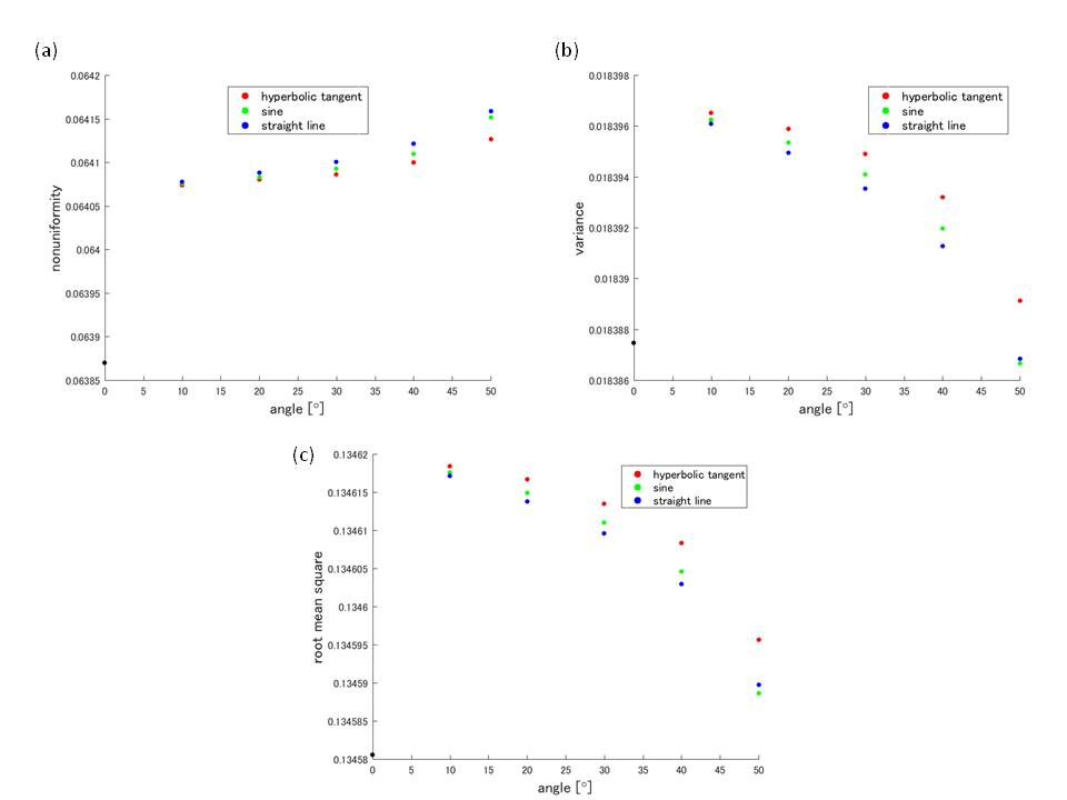
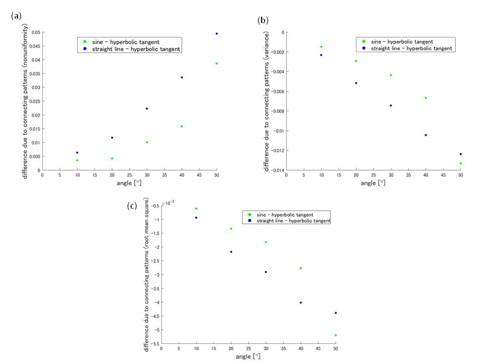
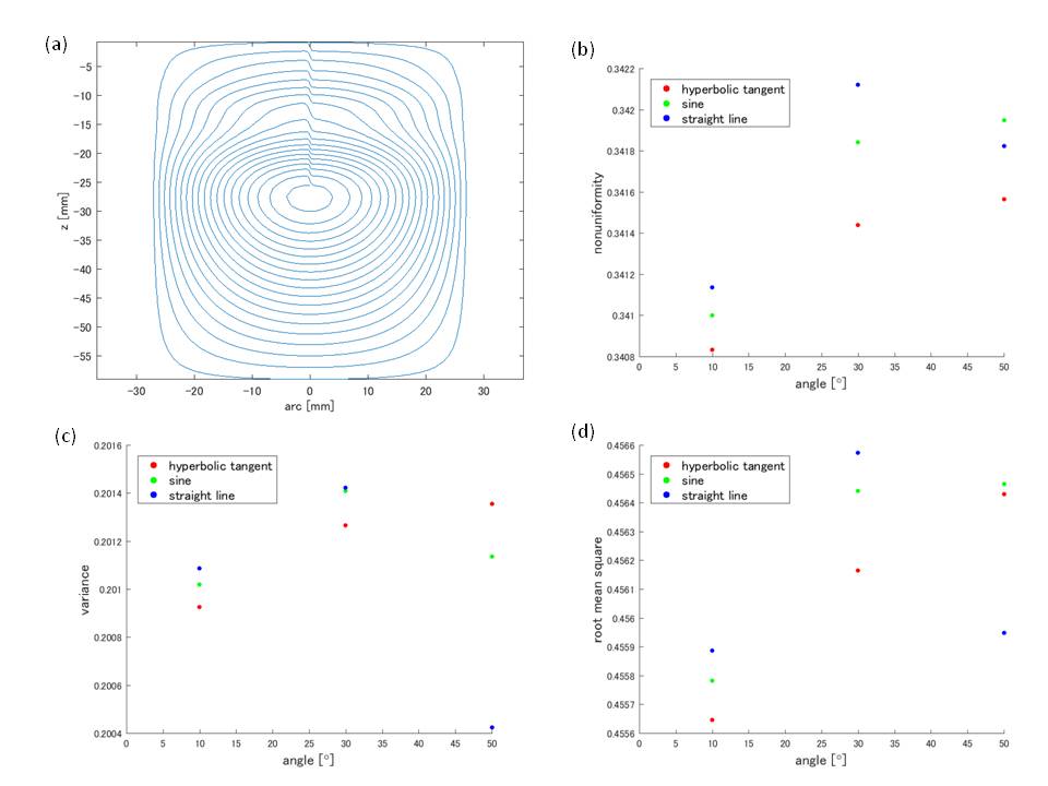
Fig. 2 shows nonuniformity (a), variance (b) and root mean square (c) about the three connecting patterns with the outside return path. The values of nonuniformity increased as the angle increased (Fig. 2 (a)). The values of variance and root mean square decreased as the angle increased (Fig. 2 (b, c)). The differences between the values of hyperbolic tangent and of sine and the values of hyperbolic tangent and of straight line are shown in Fig. 3. The absolute differences of nonuniformity, variance and root mean square gradually increased (Fig. 3 (a-c)). Around the angle of 45°, the values of the two differences in variance and root mean square became same (Fig. 3 (b, c)). In Fig. 4, three characteristics of the connecting patterns with the inside return path are shown. Due to position of the return paths, loop connections are located at the upper part of one quarter of the wire path (Fig. 4 (a)). The three characteristic values increased as the angle increased but not monotonically (Fig. 4 (b-d)).Discussion
The nonuniformity and the root mean square can be treated as L1-, L2-norms, respectively. L1-norm weighs more on smaller values, but L2-norm more on larger values. From the point of view of the gradient uniformity, smaller error is preferable. Moreover, from the construction point of view, larger angle makes winding easier. In the connecting pattern with the outside return path, therefore, employment of lager connecting angle leads to better gradient performance. Here, the nonuniformity increased with the connecting angle but the difference from the theoretical one is less than 0.5%. Since the differences between the connecting patterns become 0, robustness to pattern change may be largest at the angle of 45° even in the case that the hyperbolic tangent pattern is employed. On the other hand, in the connecting pattern with the inside return path, differences of three characteristics from the theoretical ones becomes more than three orders higher than those in the pattern with the outside return path. In the case that the wire paths are connected in the transverse direction at the angle of 20° (Fig. 5), however, the nonuniformity, the variance and the root mean square were calculated 0.0667, 0.0187 and 0.136, respectively. These findings indicate that smooth parts of the loops should be used for connecting regions. This optimization is applicable to gradient coils of larger size due to its scalability.Conclusion
We optimized the connecting pattern to have the 45° hyperbolic tangent connection with the outside return path, the optimized wire paths give us easiness of construction and smaller variance.Acknowledgements
This work was supported by JSPS KAKENHI Grant Number 17H04262.References
1. Poole M, and Bowtell R,. Novel Gradient Coils Designed Using a Boundary Element Method. Concepts in Magnetic Resonance Part B. 2007;31B(3):162-175.Figures