Introduction

Permanent magnet array is a good candidate for providing the main magnetic field for a low-field portable MRI system. Halbach array is popular in such a system. However, it provides magnetic fields that are transverse to the bore and therefore, RF coils have to be re-engineered to fit in [1,2]. A yokeless magnet array with a pair of rings that provides longitudinal field has intrinsic compatibility to existing RF coils [3]. However, the homogeneities of the magnetic field generated are not enough for MRI imaging in a large volume, for example, human head. In this abstract, we present the design of a new yokeless permanent magnet array that generates a longitudinal $$$\bf{B_0}$$$ field with significant improvement in field strength and in homogeneity compared to the traditional two-ring structure. The design and optimization was done for a portable MRI system using a current model and genetic algorithm (GA).

Methods

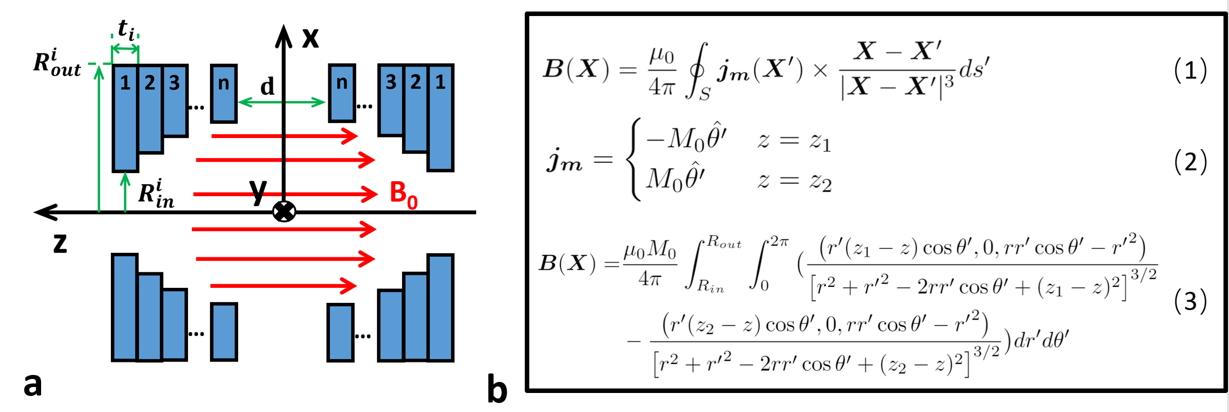
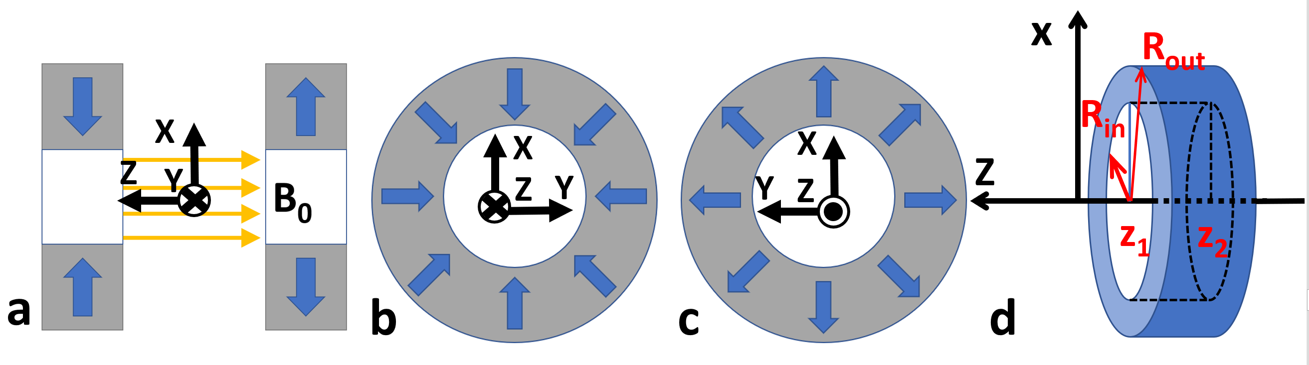
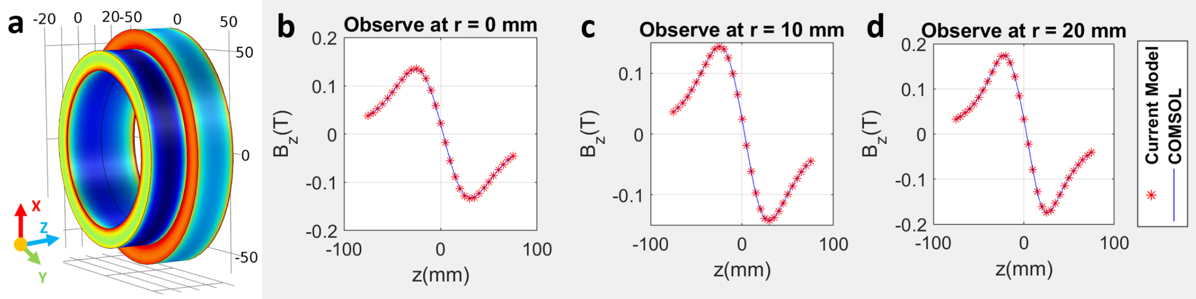
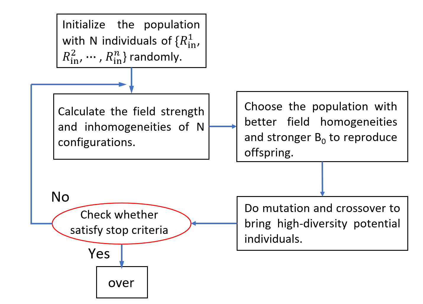
The design is an assembly of $$$n$$$ pairs of symmetric magnet rings with the axis of the rings aligned with the $$$z$$$-axis, as shown in Fig.$$$\,1$$$. Each pair of rings is the magnet assembly proposed by G. Aubert in $$$1991$$$ which generates a longitudinal field to the bore [3]. In the proposed design, as shown in Fig.$$$\,1$$$, each pair has an inner radius of $$$R_{in}^i$$$, an outer radius of $$$R_{out}^i$$$, a thickness of $$$t_i$$$, and a distance between the innermost rings of $$$d$$$. The above parameters can be optimized for field homogeneity and field strength using the GA. In order to accelerate the forward calculation of the magnetic field for optimization, a current model is applied. $$$\bf{Current}$$$ $$$\bf{Model}$$$ $$$\bf{for}$$$ $$$\bf{the}$$$ $$$\bf{Calculation}$$$ $$$\bf{of}$$$ $$$\bf{Magnetic}$$$ $$$\bf{Field:}$$$ In the current model for a single magnet ring as shown in Fig.$$$\,2(d)$$$, the magnet is reduced to the equivalent distribution of currents. Therefore, the generated magnetic field can be calculated by (1) (shown in Fig.$$$\,1$$$(b))[4], where $$$\bf{X}$$$ is the observation point, $$$\bf{X}^{\prime}$$$ is the current source point, and $$$S$$$ is the surface of the magnet. For a single magnet ring with outwards radial magnetization (shown in Fig.$$$\,2(c)$$$), the equivalent current source is shown in Eq.$$$\,(2)$$$, where $$$M_0$$$ is the magnitude of the remanent magnetization. The equivalent currents for the magnet ring in Fig.$$$\,2(d)$$$ are surface currents circulating on the front and the back surfaces of the ring.Since a magnet ring is symmetrical with respect to its radial axis, $$$\bf{B}(\bf{X})$$$ is $$$\theta$$$-independent. Therefore, the observation point is defined as $$$(r,0,z)$$$ to simplify the derivation and the calculation is reduced to a two-dimensional problem. Substitute (2) into (1) and take the integration, we get (3). It is validated by comparing with simulation results using COMSOL [5]. Fig.$$$\,$$$ 3 shows the results calculated using (3) (in MATLAB) and COMSOL. As shown, they agree with each other well. The calculation time by using (3) is about $$$1$$$ s in comparison to about $$$10$$$ s in COMSOL. The proposed approach takes much less time, thus it is ready for the forward model in optimization. $$$\bf{Genetic}$$$ $$$\bf{Algorithm:}$$$ Fig.$$$\,4$$$ shows the flowchart of GA. The parameters that are under optimization are $$$R_{in}^i$$$ $$$(i=2,...10)$$$ and the distance $$$d$$$ between the two innermost rings. The rest are preset as shown in Fig.$$$\,4$$$. The optimization criteria are field homogeneity and field strength.

Optimization Results

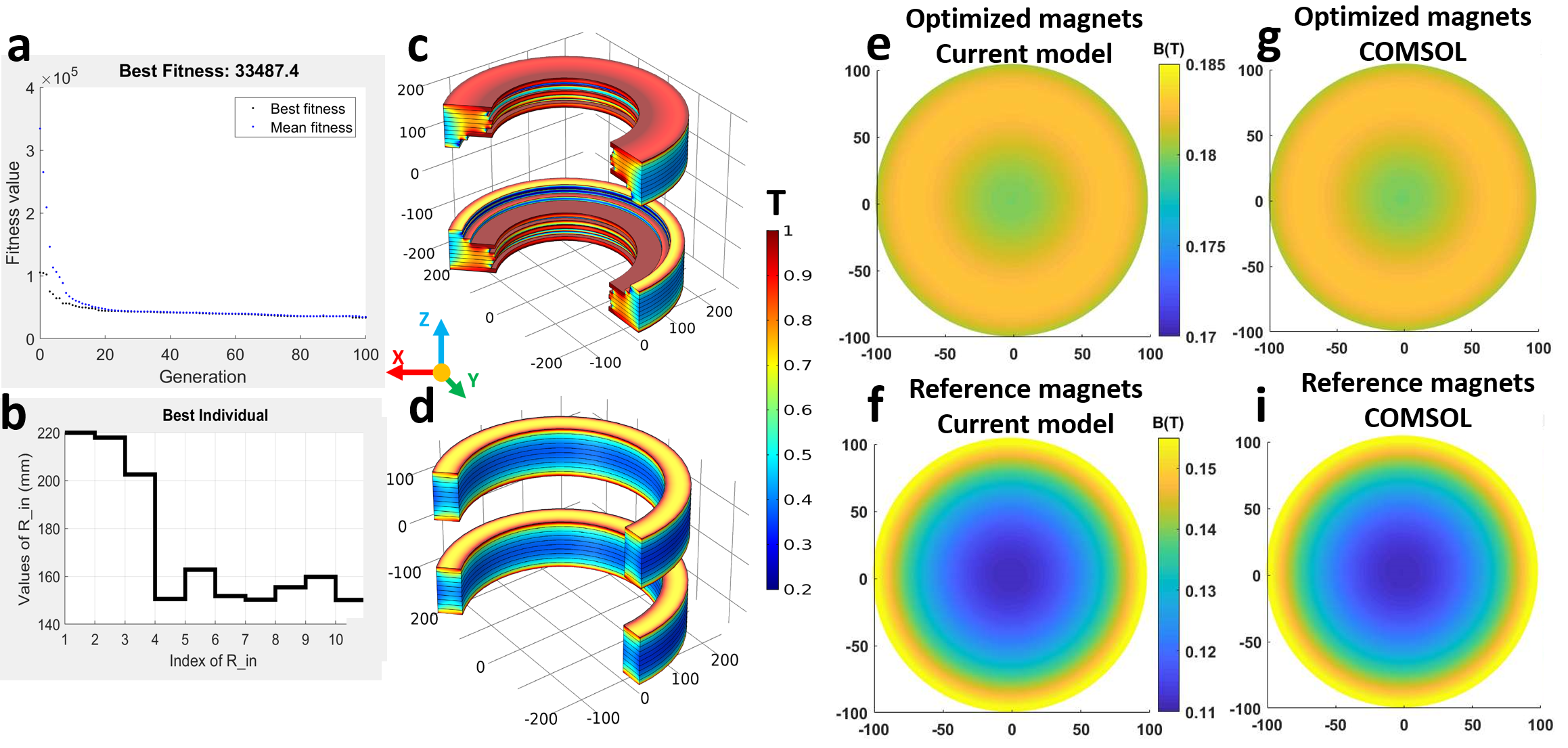
The optimization results are shown in Fig.$$$\,5$$$. A two-ring G. Aubert's configuration with a constant inner radius of 200 mm as shown in Fig.$$$\,5(d)$$$ is used as a reference. Fig.$$$\,5$$$(a) shows that the fitness value (field inhomogeneities) decreases as the number of iterations increases. Fig.$$$\,5$$$(b) shows the best $$$R_{in}^i$$$ after $$$100$$$ iterations which determines the inner profile of the optimized magnet array. The optimized array is shown in Fig$$$\,5$$$(c). Fig$$$\,5$$$(e)-(g) and (f)-(i) shows the z-components of $$$B_0$$$ on the central plane in the FOV of the optimized magnet array and that of the reference magnet, respectively, using both the current model and COMSOL. After optimization, the field inhomogeneity is greatly reduced by over $$$93\%$$$ from $$$374100$$$ ppm to $$$24687$$$ ppm in the FOV. In the meanwhile, the average field strength is increased by over $$$39\%$$$ from $$$125.9$$$ mT to $$$175.5$$$ mT in the FOV.

Conclusion

We proposed the design of a new yokeless permanent magnet array that generates a longitudinal $$$B_0$$$ field whose inhomogeneities are significantly reduced by $$$93\%$$$ and field strength is increased by $$$39\%$$$, compared to a conventional two-ring configuration [3]. The optimization was done based on a current model and GA. The effectiveness of the optimization is validated by realistic simulations using COMSOL. The optimized magnet array will be built for low-field portable MRI system in the near future.

Acknowledgements

No acknowledgement found.