1685
Obtaining the barrier distribution in the micro-structure from diffusion spectra1Department of Electrical Engineering, Pontificia Universidad Católica de Chile, Santiago, Chile, 2Biomedical Imaging Center, Pontificia Universidad Católica de Chile, Santiago, Chile, 3Division of Imaging Sciences and Biomedical Engineering, King’s College London, London, United Kingdom, 4Institute for Computational and Mathematical Engineering, Stanford University, Stanford, CA, United States, 5Institute for Biological and Medical Engineering, Pontificia Universidad Católica de Chile, Santiago, Chile
Synopsis
Inspired in the solution of the diffusion equation in the restricted case, we propose to express the diffusion $$$q$$$-space information in a restricted basis. This representation allows to obtain the distribution of barriers separations, thus providing useful information about the micro-structure. Previous methods used multiple Diffusion Spectrum Imaging (DSI) images with different diffusion times, which is impractical to characterize barriers in multiple directions. Our method proposes to obtain the barrier distribution with only a single DSI image. Furthermore, the model does not use a strong assumption for the geometry of the barriers (or axons) nor for the probability distribution of the barrier separation.
Introduction
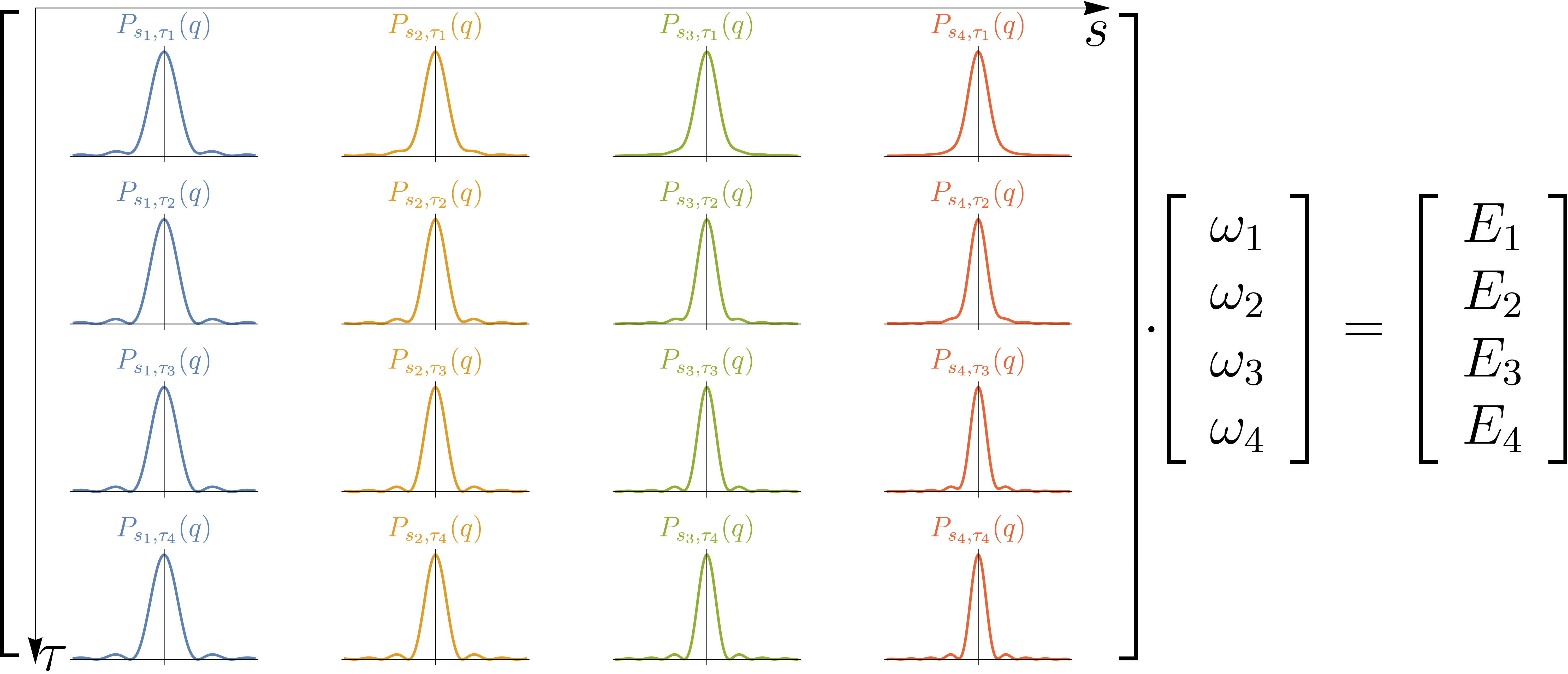
One of the aims of diffusion MRI is to characterize the obtained signal. This is typically done by fitting the data to a model or description of the signal. Examples of this are: DTI1, HARDI2 and MAP3. On the other hand there are several methods to predict the diffusion signal from physical phenomena such as CHARMED4, AxCaliber5, NODDI6. We tried to make a composition of both ways of addressing the problem. Thus, obtaining a basis with physical meaning that fits the data properly. Previous methods like AxCaliber uses multiple DSI acquisitions varying the diffusion time to retrieve the axon radii distribution, this is represented in Figure 1 where each graph represent the expected pdf for a given barrier separation and diffusion time. However, this method is time-expensive and makes the characterization in multiple angles unfeasible. Additionally, AxCaliber is based on the CHARMED model that assumes that the axon is a cylinder. Therefore, it is only possible to get information about axons.Theory
Diffusion Spectrum Imaging acquires the Fourier transform of the Ensemble Average Propagator (EAP)7,8. This is obtained theoretically by first solving the diffusion equation. The problem of interest is to solve this equation for a non-permeable enclosure of separation $$$s$$$. The mathematical formulation of this phenomena for a particle positioned at $$$x_0$$$ is described by the following differential equation and boundary conditions
$$ \begin{cases} p_{xx}=\mathrm{D}p_{t}\\ p\left(x,0\right)=\delta\left(x-x_{0}\right)\\ p_{x}\left(x,t\right)=0 & x\in\left\{ 0,\text{s}\right\} . \end{cases}$$
Solving this equation we can obtain a probability distribution (propagator) of the position of a particle which is
$$ p\left(x|x_{0}\right)=\frac{1}{s}\sqcap\left(\frac{x-s/2}{s}\right)\left[1+2\sum_{n=1}^{\infty}\cos\left(\frac{n\pi}{s}x\right)\cos\left(\frac{n\pi}{s}x_{0}\right)e^{-\mathrm{D}\Delta\left(n\pi/s\right)^{2}}\right].$$
Applying the ensemble average and then a Fourier transform we obtain the Tanner signal equation9,10
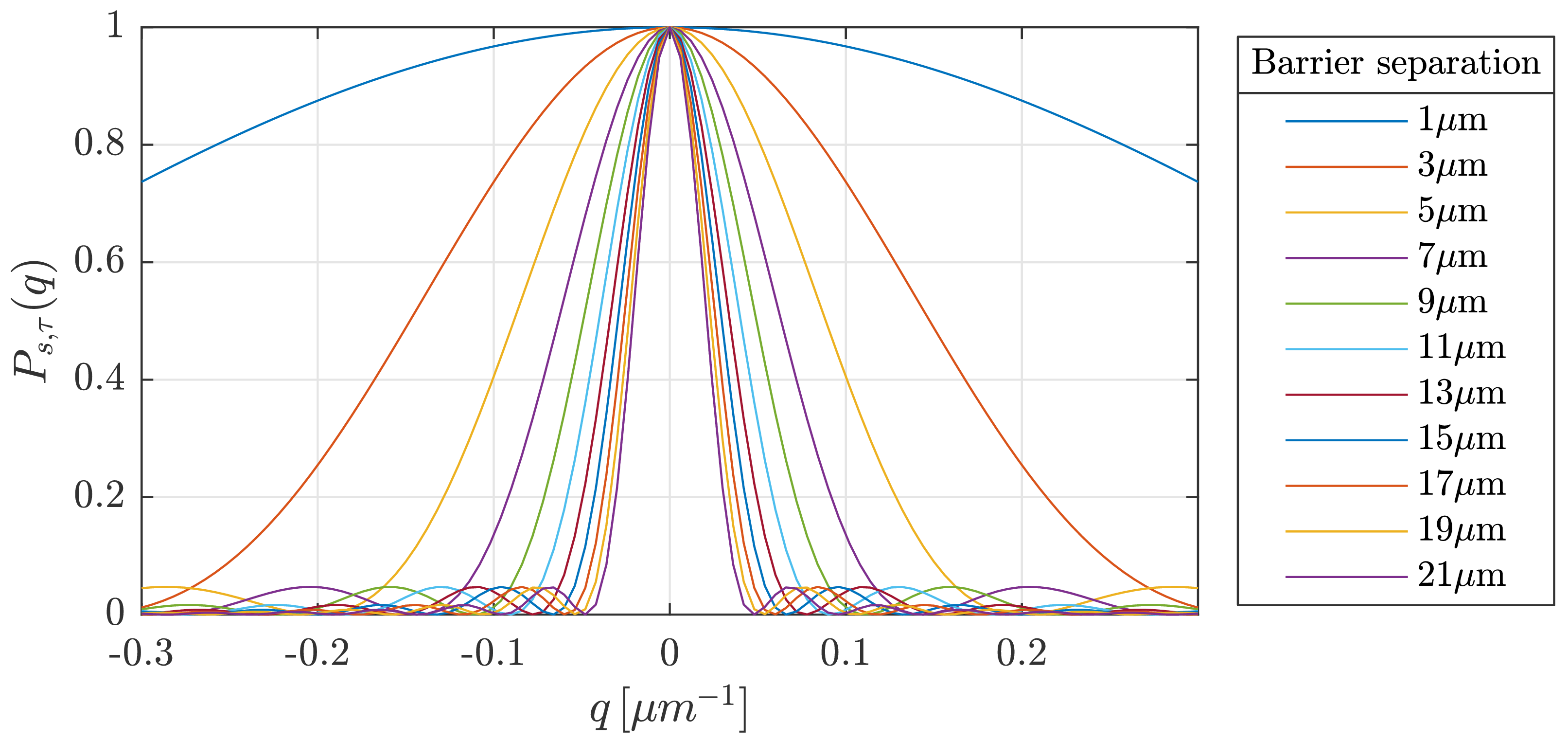
$$ P_{s,\tau}\left(q\right)=\mathrm{sinc}^{2}\left(sq\right)+2\sum_{n=0}^{\infty}\left(\frac{sq}{sq-n/2}\right)^{2}\mathrm{sinc}^{2}\left(sq+\frac{n}{2}\right)e^{-\mathrm{D}\Delta\left(n\pi/s\right)^{2}}\quad[1]\\=\sum_{n=0}^{\infty}a_{n}\left(\frac{sq}{sq-n/2}\right)^{2}\mathrm{sinc}^{2}\left(sq+\frac{n}{2}\right),\quad\quad\quad\quad\quad\quad\quad\quad$$
where we grouped the constants in $$$ a_{n}$$$. Then using $$$\left\{ P_{s,\tau}\right\} _{s\in\mathbb{R}}$$$ (as seen in Figure 2) as an atom of a dictionary we will reconstruct the barrier distribution for a given diffusion direction.
Methods
The obtained signal given a distribution of barriers is
$$ E\left(q\right)=\int_{0}^{\infty}\omega\left(s\right)P_{\tau}\left(sq\right)\mathrm{d}s\quad[2],$$
with $$$w( s )$$$ the probability distribution of finding a given barrier separation $$$s$$$. If we discretize $$$q$$$ and $$$s$$$ in [2], we obtain
$$ \vec{E}=\mathrm{P}\vec{\omega}.\quad[3]$$
Where $$$ \vec{E}$$$ is the signal in $$$q$$$-space, $$$ \mathrm{P}$$$ is a matrix representing the dictionary made from [1] and $$$\vec{\omega}$$$ is the barrier distribution. Since the linear system in [3] is not determined, we propose to solve an optimization problem using a Tikhonov regularization
$$ \hat{\omega}=\underset{\vec{\omega}}{\mathrm{argmin}}\left\Vert \mathrm{P}\vec{\omega}-\vec{E}\right\Vert _{2}+\lambda\left\Vert \vec{\omega}\right\Vert _{2}.$$
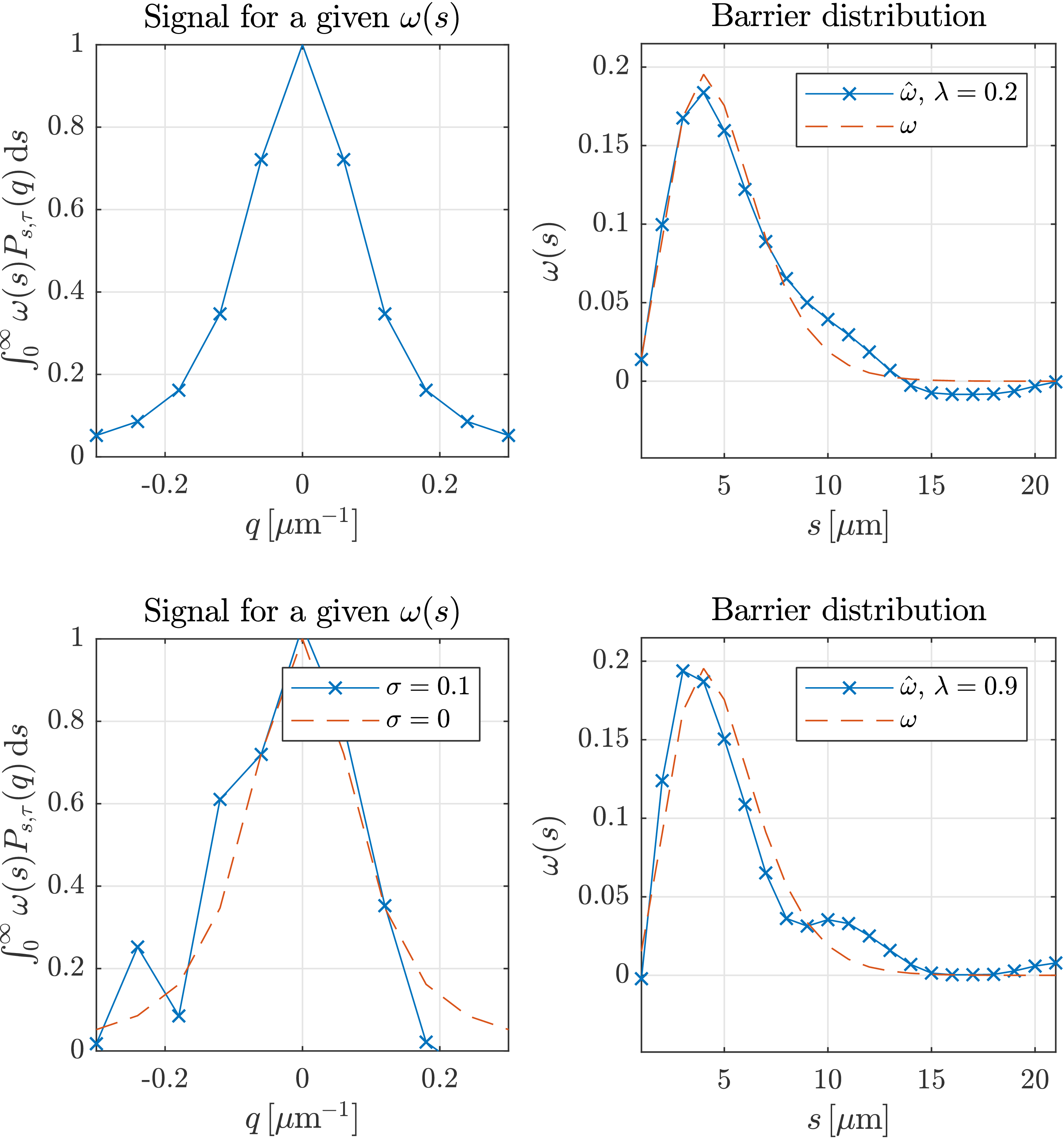
The advantage of this optimization problem is that it has a close solution $$$ \hat{\omega}=\left(\mathrm{P}^{\mathrm{T}}\mathrm{P}+\lambda^{2}\mathbb{I}\right)^{-1}\mathrm{P}^{\mathrm{T}}\vec{E}$$$. Which can be solved without the use of a complex optimization algorithm. The method was tested on a simulated signal of 11 samples with $$$ q_{\max}=0.3\mu\mathrm{m}^{-1}$$$ and a $$$ s\sim\Gamma\left(5\mu\mathrm{m},1\mu\text{m}\right)$$$ adding Gaussian noise of different standard deviations $$$\sigma$$$ . Figure 3 shows the barriers in a pixel for an instance the $$$\Gamma$$$ probability distribution.
Results and discussion
In Figure 4 we show the results on a noiseless signal in which a proper reconstruction was possible. We see similar results for a signal with noise of $$$\sigma=$$$ 10% and the behavior for different noise levels between 1-10% is shown in Figure 5. While the results are not perfect, they are promising because the number of samples in $$$q$$$-space is 11 . However it is not shown here that incrementing the number of samples decreases the NMRSE by 4%. Thus, the usage of under-sampling techniques to increase the number of data points can be explored to achieve better results.Conclusion
The proposed method was able to obtain an accurate barrier distribution without multiple acquisition at different diffusion times. The signal model is based on the 1D restricted diffusion problem which provides atoms for a dictionary. Consequently, we provide a model that is able to represent the signal only assuming non-permeable barrier without any other supposition of the geometry nor barrier separation distribution. The ongoing research will continue to explore other regularization methods to do an analysis in multiple directions on 3D-DSI data.Acknowledgements
The authors gratefully acknowledge CONICYT for funding this research through PIA-Anillo ACT1416.References
1. Le Bihan D, Mangin J-F, Poupon C, Clark CA, Pappata S, Molko N, Chabriat H. Diffusion tensor imaging: Concepts and applications. Journal of Magnetic Resonance Imaging. 2001;13(4):534–546. doi:10.1002/jmri.1076
2. Berman JI, Lanza MR, Blaskey L, Edgar JC, Roberts TPL. High Angular Resolution Diffusion Imaging (HARDI) Probabilistic Tractography of the Auditory Radiation. AJNR. American journal of neuroradiology. 2013;34(8):1573–1578. doi:10.3174/ajnr.A3471
3. Özarslan E, Koay CG, Shepherd TM, Komlosh ME, İrfanoğlu MO, Pierpaoli C, Basser PJ. Mean apparent propagator (MAP) MRI: A novel diffusion imaging method for mapping tissue microstructure. NeuroImage. 2013;78:16–32. doi:10.1016/j.neuroimage.2013.04.016
4. Assaf Y, Basser PJ. Composite hindered and restricted model of diffusion (CHARMED) MR imaging of the human brain. NeuroImage. 2005;27(1):48–58. doi:10.1016/j.neuroimage.2005.03.042
5. Assaf Y, Blumenfeld-Katzir T, Yovel Y, Basser PJ. AxCaliber: A Method for Measuring Axon Diameter Distribution from Diffusion MRI. Magnetic resonance in medicine. 2008;59(6):1347–1354. doi:10.1002/mrm.21577
6. Zhang H, Schneider T, Wheeler-Kingshott CA, Alexander DC. NODDI: Practical in vivo neurite orientation dispersion and density imaging of the human brain. NeuroImage. 2012;61(4):1000–1016. doi:10.1016/j.neuroimage.2012.03.072
7. Callaghan P, MacGowan D, Packer KJ, Zelaya FO. Influence of field gradient strength in NMR studies of diffusion in porous media. Magnetic Resonance Imaging. 1991;9(5):663–671. doi:10.1016/0730-725X(91)90355-P
8. Callaghan PT. Principles of Nuclear Magnetic Resonance Microscopy. Clarendon Press; 1993.
9. Tanner JE, Stejskal EO. Restricted Self‐Diffusion of Protons in Colloidal Systems by the Pulsed‐Gradient, Spin‐Echo Method. The Journal of Chemical Physics. 1968;49(4):1768–1777. doi:10.1063/1.1670306
10. Stejskal EO, Tanner JE. Spin Diffusion Measurements: Spin Echoes in the Presence of a Time‐Dependent Field Gradient. The Journal of Chemical Physics. 1965;42(1):288–292. doi:10.1063/1.1695690
Figures