1651
Deep learning with synthetic data for free water elimination in diffusion MRI1Technical University of Munich, Munich, Germany, 2GE Global Research Europe, Munich, Germany
Synopsis
Diffusion metrics are typically biased by Cerebrospinal fluid (CSF) contamination. In this work, we present a deep learning based solution to remove the CSF contribution. First, we train an artificial neural network (ANN) with synthetic data to estimate the tissue volume fraction. Second, we use the resulting network to predict estimates of the tissue volume fraction for real data, and use them to correct for CSF contamination. Results show corrected CSF contribution which, in turn, indicates that the tissue volume fraction can be estimated using this joint data generation and deep learning approach.
Introduction
Cerebrospinal fluid (CSF) partial volume contamination poses a problem for detecting changes in tissue microstructure1, biasing the diffusion measurements and derived metrics. CSF is mostly composed of free water, with isotropic diffusion and diffusivity three times bigger than parenchyma2.
FLAIR DWI3 tackles the problem suppressing the CSF signal during acquisition, at the cost of low SNR and longer acquisition times. Post-processing solutions have focused on fitting a bi-tensor model; yet, this is an ill-posed problem with several regularizations1,2,4-7.
In this work, we hypothesise and show that artificial neural networks (ANN) can estimate the tissue volume fraction from the diffusion signal. Then the CSF contribution can be corrected.
Methods
Theory
CSF has isotropic diffusion with diffusivity $$$D_{CSF}=3·10^{-3}mm^2/s$$$ 2 and can be computed from b:
$$S_{CSF}=e^{-b·D_{CSF}}. $$[Eq.1]
The measured signal is the contribution of CSF and tissue (parenchyma) components:
$$S = fS_{tissue} + (1-f)S_{CSF}.$$ [Eq.2]
Eq.2 is ill-posed since $$$S_{tissue}$$$ and its volume fraction, $$$f$$$, are unknowns. In this work, we present a deep learning approach that uses ANNs to estimate $$$f$$$, regularizing the problem:
$$S_{tissue} = \frac{S-(1-f)S_{CSF}}{f}.$$ [Eq.3]
Generation of synthetic data
The training dataset were designed to teach the ANN to detect CSF-like components mixed with a random signal (Fig.1). CSF signal was derived from Eq.1 and acquisition parameter b. Tissue signal was randomly generated to simulate undetermined directions. The generation steps were:
- $$$S_{CSF}^{training}$$$ was computed (Eq.1).
- $$$S_{tissue}^{training}$$$ was randomly created simulating arbitrary directions: $$$U(0,1)$$$.
- $$$f$$$ was randomly generated: $$$U(0,1)$$$.
- $$$S^{training}$$$ was computed (Eq.2).
- The ANN was trained with input $$$S^{training}$$$ to match the output $$$f$$$ (Fig.2).
Free water elimination
For comparison, we trained10 five ANN architectures in MATLAB (MathWorks, Natick, MA) for datasets with 32 directions (one shell) and 64 directions (two shells), (Fig.2). We chose the best performing ANNs and compared them against Pasternak's4 and Hoy’s6,11 methods.
Data acquisition
A volunteer went under a diffusion acquisition (GE 3T MR750w, Milwaukee, WI) with 30 directions and 2 shells: b=500, 1000s/mm2; four b=0s/mm2; TR/TE=8000/80ms; FOV=200mm; resolution 128x128; ASSET=2; and 25 slices with 3.6mm thickness and no gap.
Pipeline
- Diffusion measurement.
- Synthetic data generation from the experimental b (Fig.1).
- ANN training.
- Volume fraction estimation: $$$f=ANN(S)$$$.
- Computation of $$$S_{tissue}$$$ (Eq.3).
- Fitting of the tensor model8,9 on $$$S_{tissue}$$$.
Results
The five ANN architectures (Fig.2) showed similar performance (Fig.3). ANNs trained for two shells (ANN2s) outperformed those for one shell (ANN1s), due to the better CSF encoding of two shells protocols. The best performing ANNs were L=2 and L=3 for one and two shells respectively, suggesting a potential coupling between the number of hidden layers and shells.
DTI metrics after ANNs correction showed differences depending on the number of shells. ANN1s estimated larger volumes of CSF than ANN2s (Fig.4c), that resulted in larger FA (Fig.4a) and lower MD (Fig.4b) estimates. This difference on the $$$f$$$ estimate might be explained by the limited CSF information contained in the single shell protocol. MD values for ANN2s (Fig.4b) agreed with the reference2.
ANNs kept the anatomical integrity of the FA, MD, and $$$f_{CSF}$$$ maps (Fig.5). We observed the CSF correction in the enlargement of the corpus callosum and fornix, and a general increment of FA in white matter, compared to the standard DTI (Fig.5a,c,e,f). CSF contribution was accurately removed from MD maps, especially for ANN2s (Fig.5g,h,k,l). ANNs1 and ANNs2 differ on the $$$f$$$ estimate in white matter (Fig.5m,o), as previously explained.
Discussion
ANNs trained with synthetic data are capable of estimating the tissue volume fraction from the measured diffusion signal. Their correction is equivalent to well-established methods: Pasternak et al4. and Hoy et al6. (Fig.4 and Fig. 5).
Using ANNs has a performance advantage. Their training time is in the order of ten minutes and once trained they can be used for any data acquired with the same protocol. CSF correction is faster than traditional methods. For one shell, Pasternak’s method ran for 38.4s and ANN1s for 0.7s (55x). For two shells, Hoy’s method ran for 392.5s and ANN2s for 1.3s (302x). Besides, to improve the accuracy, one can carefully design the training dataset to mimic only tissue characteristics (here it is random), or incorporate prior knowledge of the bi-exponential problem and noise model into the learning process12.
Conclusions
This is the first application of ANNs to remove CSF contamination. We proved that tissue volume fraction can be estimated by ANNs trained with synthetic data, creating a new tool for free water elimination.Acknowledgements
With the support of the TUM Institute of Advanced Study, funded by the German Excellence Initiative and the European Commission under Grant Agreement Number 605162.References
1 C. Metzler-Baddeley, M. J. O’Sullivan, S. Bells, O. Pasternak, and D. K. Jones, “How and how not to correct for CSF-contamination in diffusion MRI.,” Neuroimage, vol. 59, no. 2, pp. 1394–403, Jan. 2012.
2 C. Pierpaoli and D. K. Jones, “Removing CSF Contamination in Brain DT-MRIs by Using a Two-Compartment Tensor Model,” in Proceedings of the 12th Annual Meeting of ISMRM, Kyoto, 2004, p. 1215.
3 G. Liu, P. Van Gelderen, J. Duyn, and C. T. W. Moonen, “Single-shot diffusion MRI of human brain on a conventional clinical instrument,” Magn. Reson. Med., vol. 35, no. 5, pp. 671–677, 1996.
4 O. Pasternak, N. Sochen, Y. Gur, N. Intrator, and Y. Assaf, “Free Water Elimination and Mapping from Diffusion MRI,” vol. 730, pp. 717–730, 2009.
5 Z. Eaton-Rosen, A. Melbourne, M. J. Cardoso, N. Marlow, and S. Ourselin, “Beyond the Resolution Limit: Diffusion Parameter Estimation in Partial Volume,” MICCAI 2016, vol. 1, pp. 605–612, 2016.
6 A. R. Hoy, C. G. Koay, S. R. Kecskemeti, and A. L. Alexander, “Optimization of a Free Water Elimination Two-Compartment Model for Diffusion Tensor Imaging,” Neuroimage, no. 103, pp. 323–333, 2014.
7 M. Molina-Romero, P. A. Gómez, J. I. Sperl, A. J. Stewart, D. K. Jones, M. I. Menzel, and B. H. Menze, “Theory, validation and application of blind source separation to diffusion MRI for tissue characterisation and partial volume correction,” in Proceedings of the 25th Annual Meeting of ISMRM, Honolulu, 2017, p. 3462.
8 P. J. Basser, J. Mattiello, and D. LeBihan, “MR diffusion tensor spectroscopy and imaging.,” Biophys. J., vol. 66, no. 1, pp. 259–267, 1994.
9 M. Jenkinson, C. F. Beckmann, T. E. J. Behrens, M. W. Woolrich, and S. M. Smith, “FSL,” Neuroimage, vol. 62, no. 2, pp. 782–790, 2012.
10 M. T. Hagan and M. B. Menhaj, “Training Feedforward Networks with the Marquardt Algorithm,” IEEE Trans. Neural Networks, vol. 5, no. 6, pp. 989–993, 1994.
11 E. Garyfallidis, M. Brett, B. Amirbekian, A. Rokem, S. van der Walt, M. Descoteaux, and I. Nimmo-Smith, “Dipy, a library for the analysis of diffusion MRI data,” Front. Neuroinform., vol. 8, 2014.
12 J. Adler and O. Öktem, “Solving ill-posed inverse problems using iterative deep neural networks,” no. 1, pp. 1–24, 2017. arXiv:1704.04058v2
Figures
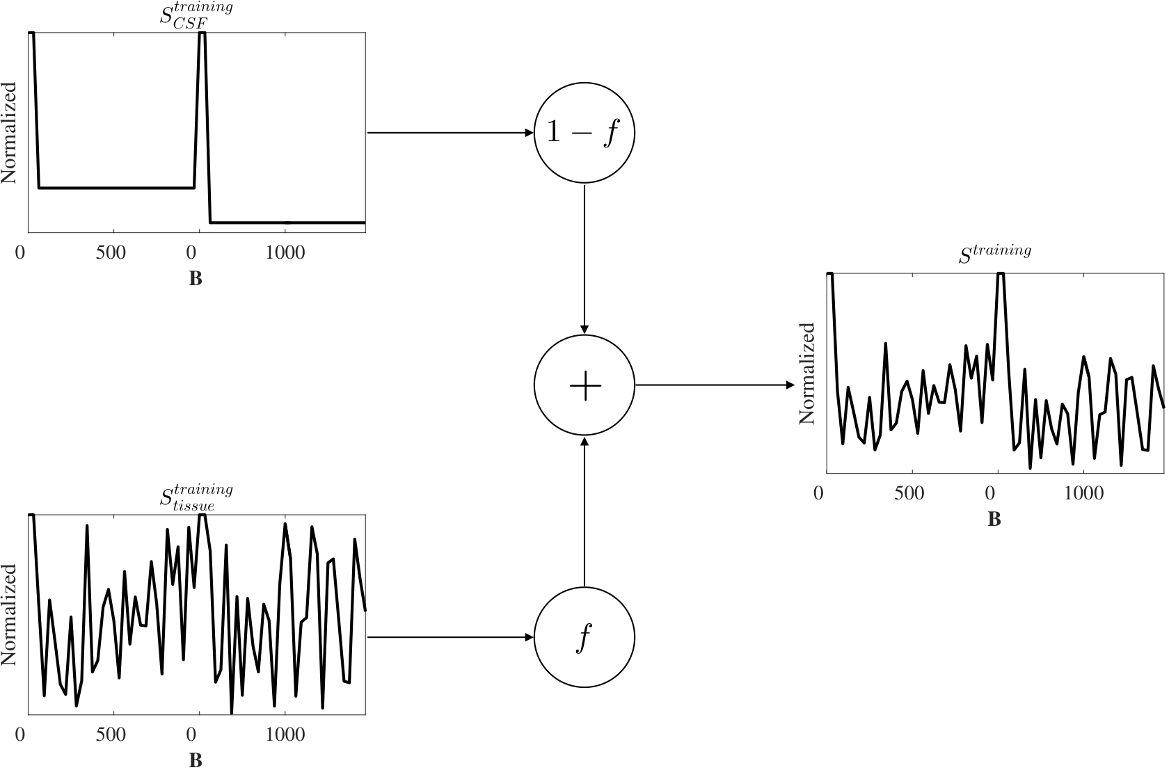
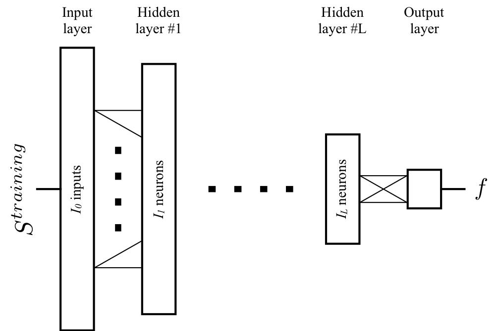
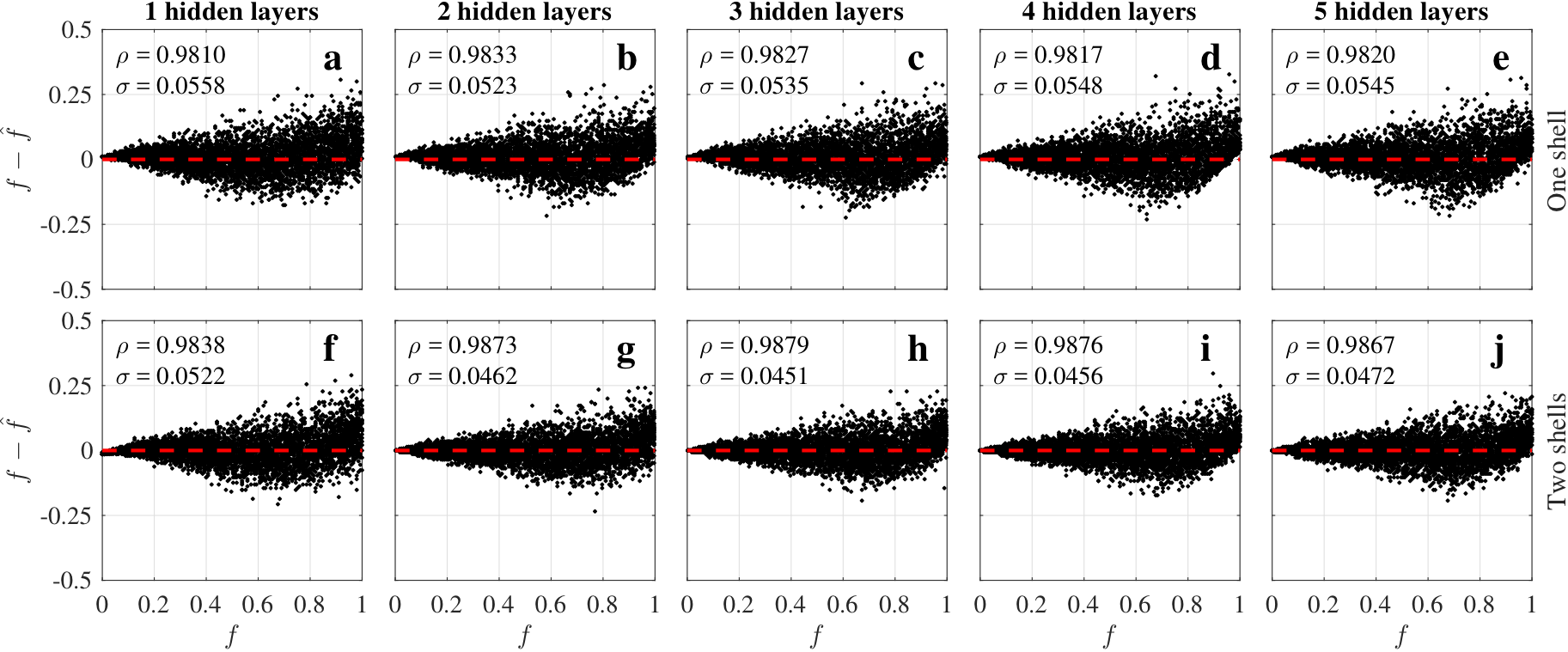
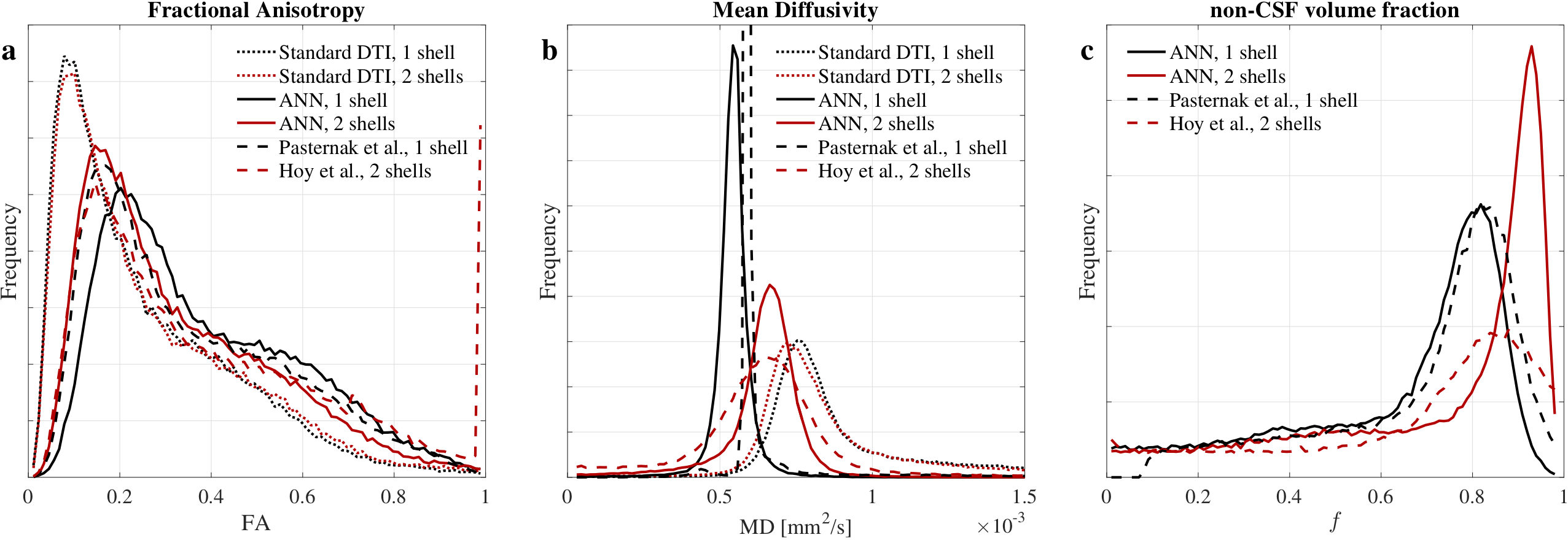
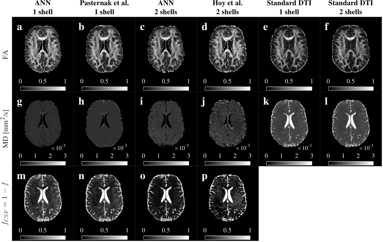
Fig.5 Comparison of FA, MD and $$$f_{CSF}$$$ maps. ANN’s maps showed anatomical coherence with standard DTI, Pasternak’s and Hoy’s methods. We observed an enlargement of the corpus callosum and recovery of the fornix in FA for all the methods (a-d) comparted to the standard (e-f). CSF contribution was removed from all the MD maps (g-j vs k-l). MD maps for two shells methods (i-j) contained more information than one shell (g-h). Single shell methods (m-n) showed a larger CSF volume estimate in white matter. ANN2s estimated a lower and more homogeneous CSF volume (o) than Hoy’s (p) in white matter.