1650
The Determination of Voxel Anisotropic Properties From Data of Low Agular Resolution Using Machine Learning Method and Compressed Sensing Reconstruction1School of Computer Science and Technology, Beijing Institute of Technology, Beijing, China, 2Center for Biomedical Imaging Research, Department of Biomedical Engineering, Tsinghua University, Beijing, China, 3Department of Biomedical Engineering, School of Medicine, Tsinghua University, Beijing, China
Synopsis
The estimation of voxel anisotropic properties from diffusion tensor imaging is critical for fiber tracking. Here machine learning was used to estimate the voxel anisotropic properties from undersampled data that were reconstructed by dictionary learning.
Purpose:
The estimation of voxel anisotropic properties from diffusion tensor imaging is critical for fiber tracking. There have been several models to compute the anisotropic properties. For example, Gaussian model can be used in the common diffusion tensor calculation; Mutil-tensor model can be used for fiber crossing or more complicated situations. These models have both advantages and disadvantages. One hypothesis is that using different or suitable models in different regions may provide improved accuracy. However, in practice, it is not feasible to apply different models to calculate voxel anisotropic properties in different places. Machine learning[1] may be helpful to address these complicated issues providing that optimally processed data exists. This study aims to investigate the feasibility of machine learning method in simple situations. After finishing learning, the model can be extended to reconstruct and analyze different and complex properties. Furthermore, the feasibility to accelerate data acquisition using the proposed model is explored, which is useful in clinical application.Methods:
A bridge is prepared between the experiment results and the input of training data. First, DTI images are transformed to a spherespace, which is similar to q-space, and E(q) is obtained. Here we used a 7×7×7 space to simulate the sphere. Then E(q) can be expressed by a space here:
$$E\left( q \right) =\int_{r\in R^3}{S_{PDF}\left( r \right) \exp \left( -2\pi iq\cdot r \right) dr}\ Eq.1 $$
Here E is the DWI data with q directions in the sphere space; r is the radial length in the sphere space. SPDF is probabilistic density function,where S is like PDF but not exactly PDF in diffusion spectrum imaging (DSI). We define this value as SPDF, where S means similar but not the same as PDF. SPDF is the input data for the machine learning, and can be computed by inverse Fourier transform of E. Alexander et al once presented a voxel-classify computing method to estimate the anisotropy of each voxel[2,3]. Here we use the same computing method to compute the voxel anisotropy properties as the reference. With SPDF and the voxel properties prepared, machine learning based on neural network is performed. Then the achieved neural network isused for new input data to get voxel properties.
Next the SPDF computing model is applied to the undersampled datasets.Here we use compressed sensing (CS) (Eq. 2) combined with sparse dictionary[4], calculated by (Eq. 3)
$$\min _{S_{PDF}}\left| F_{\Omega}\left( S_{PDF} \right) -E \right|_1+\alpha |S_{PDF}|_1\ Eq.2 $$
$$\min _{S_{PDF},D}\sum_{i=1}^n{\left| x_i \right|_0}\ s.t.\left| S_{PDF}-DX \right|_{F}^{2}\le \epsilon\ Eq.3$$
where E denotes the corresponding undersampled sphere space data, α is the regularization parameter, x is transform coefficient vectors with ncolumns, F is the Frobenius norm , D is the dictionary matrix. The SPDF values can then be used in the machine learning to obtain the voxel properties. The SPDF values of reconstructed results are compared with the CS L1-norm (Eq. 2) and the direct Fourier methods. RMSE is calculated for the comparison.
Results and Discussion:
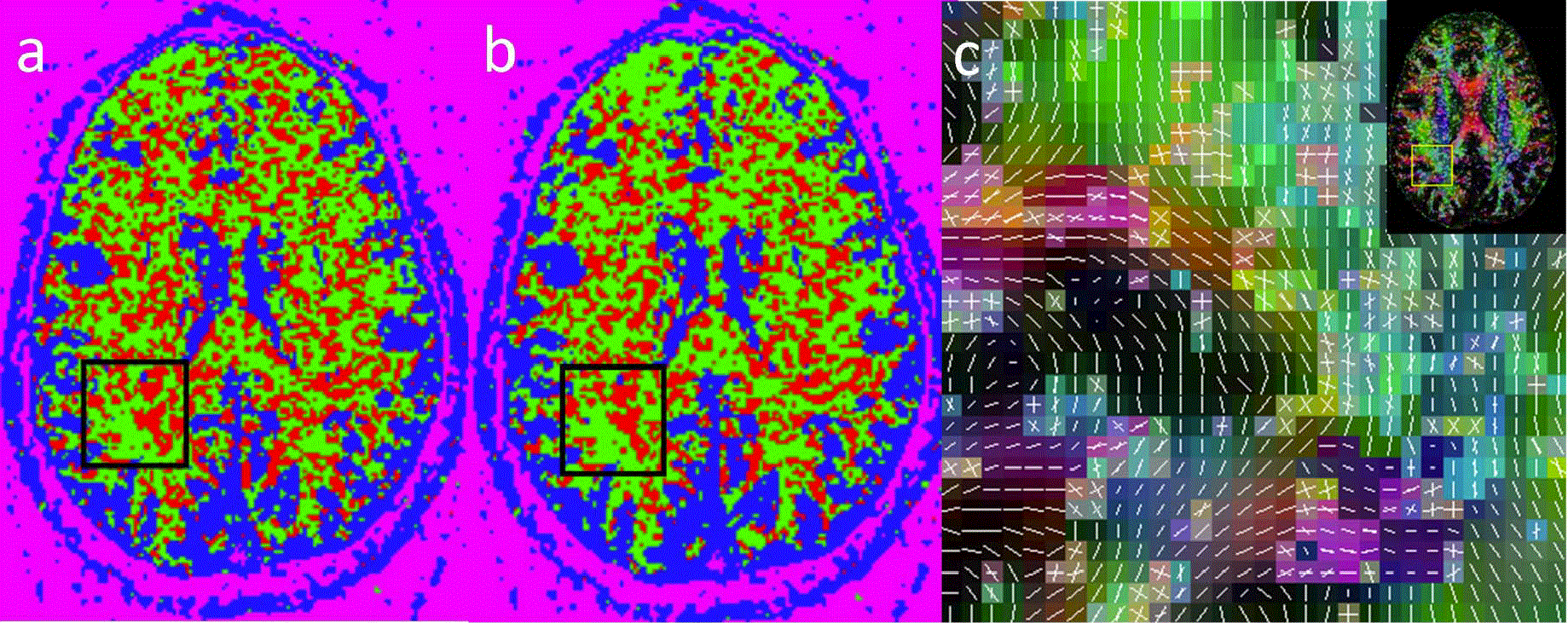
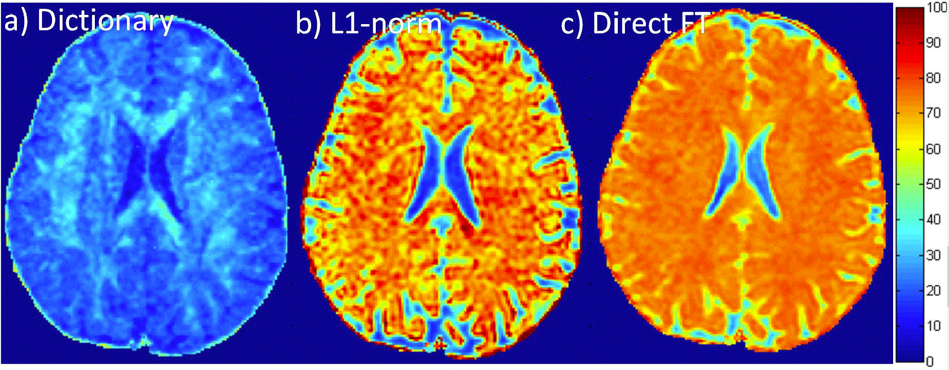
Fig.1 shows results from the machine learning. As shown in Fig. 1a and 1b, the highlighted area within the black box, the results from machine learning are comparable to the results based on Alexander's method. The related tensor fit from the black box is shown in Fig. 1c. These results indicate that our machine learning method can also be used to estimate voxel anisotropy properties. Fig. 2 shows RMSE maps for results with 3 fold undersampling. Compared with the dictionary learning in Fig. 2a, L1-norm reconstruction in Fig. 2b and direct Fourier transform in Fig. 2c present much higher reconstruction errors. So the dictionary learning is better than other two. Therefore, the SPDF value reconstructed from the CS-based dictionary learning is more precise and could be used to the machine learning. The machine learning is an efficient way for estimating the voxel anisotropy properties, especially for the complex situations in different voxels when they cannot be computed identically. Machine learning can fill up the gap and fully use of the knowledge of the known voxel properties. Furthermore, when DTI data is undersampled, by using CS and dictionary combined method, the reconstructed results can also be used in the machine learning. Here only 25-direction DTI data were used as the training data, If more directions (e.g., HARDI or DSI) are used, the successful learning ratio can help to achieve more improvement.Conclusion:
In this work machine learning was used to estimate the voxel anisotropic properties from undersampled data that were reconstructed by dictionary learning.Acknowledgements
No acknowledgement found.References
[1] R.B.Palm, IMM, 2012. [2] P.A.Cook, et.al, 14th ISMRM, 2006.[3]Camino: http://cmic.cs.ucl.ac.uk/camino//index.php?n=Main.Citations. [4] Bilgic, B et.al, MRM, 2012.Figures