Synopsis

Mean apparent propagator (MAP) reconstructs the diffusion pdf using a dictionary based on Hermite functions. The first element corresponds to a tensor approximation; and the following elements add non-gaussian components. To improve non-gaussian accuracy, one needs to increase the size of the dictionary, but it also increases the number of q-space samples for a robust optimisation. We propose the use of compressed sensing to efficiently increase the number of atoms in the dictionary by exploiting its sparsity for a better reconstruction.

Purpose

Introduction

The mean apparent propagator (MAP) ^1,2 reconstruction optimises the weights, $$$ \mathbf{x} $$$, of its dictionary to find the best fit to the q-space signal,

$$ \min || \Phi (\mathbf{A},\mathbf{q}) \mathbf{x} - P(\mathbf{q}) ||_2^2\ \ \ [1], \\ \textrm{s.t}\ \Psi (\mathbf{A},\mathbf{r}) \mathbf{x} \geq 0 \ \ \ $$

where $$$ \Phi (\mathbf{A},\mathbf{q}) $$$ is the dictionary in q-space, $$$ \Psi (\mathbf{A},\mathbf{r}) $$$ is the dictionary in the diffusion propagator space; and the scaling tensor $$$ \mathbf{A} $$$ is used to scale the atoms of both dictionaries. Normally, the dictionaries are truncated to the first 50 atoms; however, it may be insufficient to describe complex microstructures. To overcome this, the length of the dictionary needs to be increased, though it also requires more q-space samples for a robust optimisation. We propose to use compressed sensing to find the weights from a larger dictionary while using a reduced number of samples.

Theory

Given the sparse weighting of the dictionary ², we propose a MAP reconstruction based on compressed sensing ³; hence,

$$ \min\ || \mathbf{x} ||_1 \ \ \ [2], \\ \textrm{s.t} \ || SF\Psi (\mathbf{A},\mathbf{r}) \mathbf{x} - P(\mathbf{q}) ||_2^2 \leq \epsilon$$

where $$$ SF $$$ is the undersampled Fourier operator; and the error in the data consistency term is proportional to the noise in the data.

Methods

MAP vs MAP-CS

A comparison was done between [1] and [2]. For MAP, we used 50 atoms as in ^1,2. For MAP-CS, we used an extended dictionary with 161 atoms. The CS implementation was done using SPGL1 ^4,5.

To obtain $$$ \mathbf{A} = \textrm{diag}({\mu _x}^2, {\mu _y}^2, {\mu _z}^2) $$$ for both methods, we first fitted the diffusion tensor, $$$ \textrm{D}(\mathbf{q},\Delta)=\textrm{exp}(-4\pi^{2}\Delta\mathbf{qDq}^{T}) $$$, in its eigen decomposition $$$ \mathbf{D}=Q(\vec{\mathbf{\theta}})\Lambda(\vec{\mathbf{\lambda}})Q(\vec{\mathbf{\theta}})^{T} $$$ to constrain $$$\vec{\mathbf{\lambda}}$$$ and $$$\vec{\mathbf{\theta}}$$$. Second, a dilated version of the atoms as in ^1,2 was used; thus, $$$\mathbf{\mu}_{\{x,y,z\}}=2\pi\sqrt{\beta 2 \lambda_{\{x,y,z\}} \Delta}$$$ and $$$\beta=0.5$$$ in order to generate the atoms of each dictionary.

Data

The simulated data was generated using Camino software ^6,7 for two-crossing fibres with 60° and 90° angles. We added Gaussian noise to the simulated measurements in the real and imaginary channel to simulate $$$\textrm{SNR}=10$$$.

The fully sampled q-space data was retrospectively undersampled in order to apply each reconstruction method. For MAP, we used one fourth of the data (64 samples); For MAP-CS, we used one eighth of the data (32 samples).

We also acquired real data from a 60° diffusion phantom ⁸, using $$$\delta =31~\textrm{ms}$$$ and $$$\Delta =39~\textrm{ms}$$$; thus, $$$q_{\textrm{max}} = 73.64~\textrm{mm}^{-1}$$$. The scan was done with $$$\textrm{TE} =139~\textrm{ms}, \textrm{TR}=2~\textrm{s}$$$ and resolution $$$2.0 \textrm{x} 2.0 \textrm{x} 3.0~\textrm{mm}^3$$$.

Quality Indexes

To quantitatively evaluate the reconstructions against the ground truth (fully sampled), we used the normalised-root-mean-squared-error (NRMSE) and the Pearson's correlation coefficient (PC).

Results

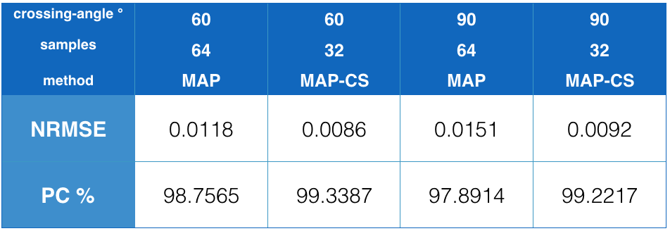
Figure 1 shows the indexes for the 60° and 90° crossing-angle reconstructions.

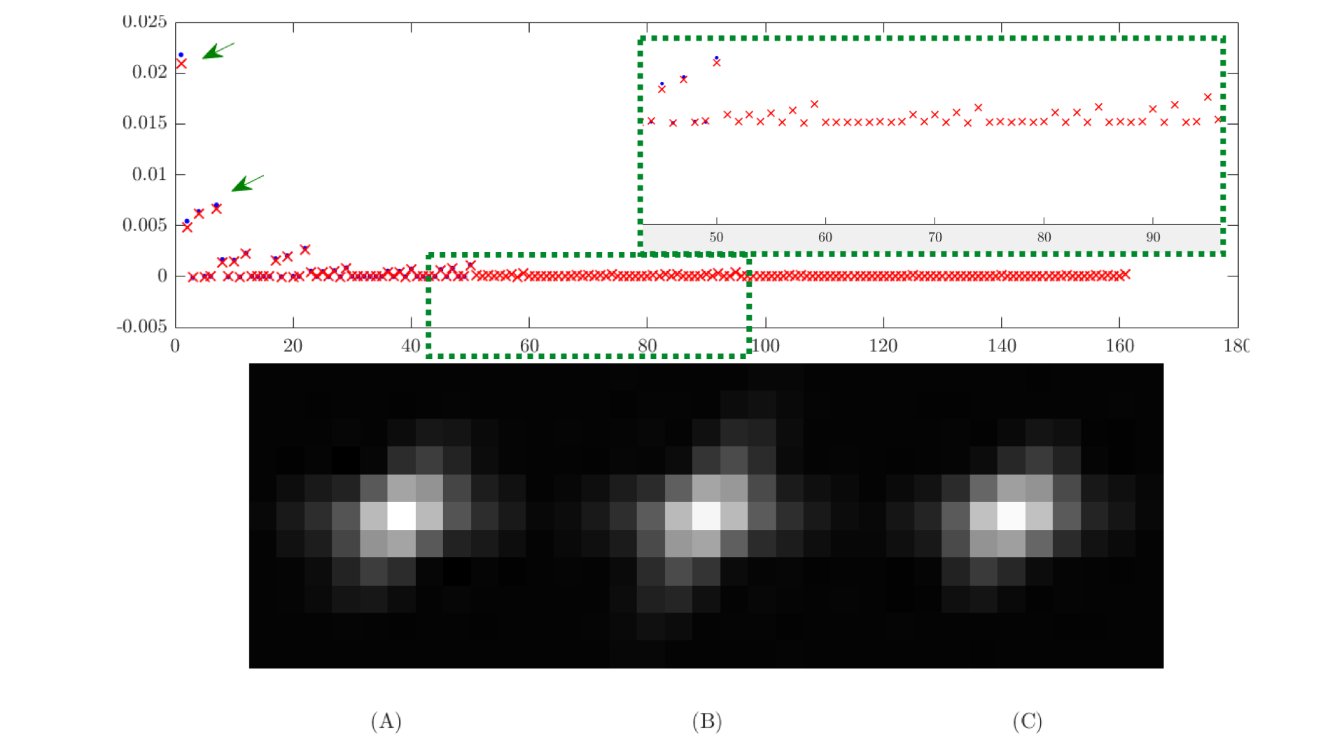
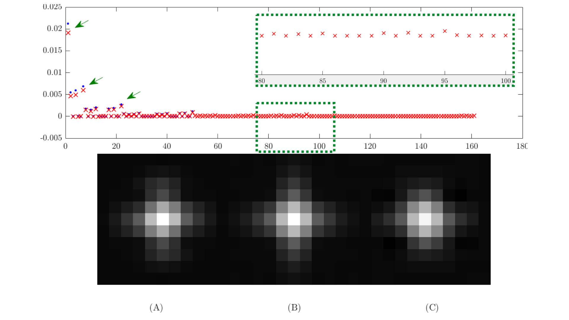
Figure 2 and 3 show the weights for each element of the dictionary for the 60° and 90° noisy simulations and their respective reconstructions. The weights are similar in both reconstructions; however, the weighting from the additional atoms makes an improvement in the reconstruction quality. There is also a reduction in the weights of the first atoms.

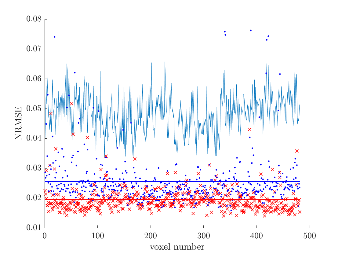
Figure 4 shows the NRMSE from the reconstruction for each voxel in the diffusion phantom. MAP-CS has a lower NRMSE when compared to MAP.

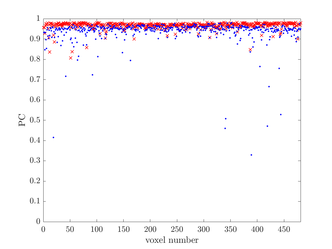
Figure 5 shows the PC from the reconstruction for each voxel in the diffusion phantom. The MAP-CS proposal has a higher PC when compared to MAP.

Conclusion

Given the sparse representation of the weights in the dictionary, we propose a CS-based MAP reconstruction. Quality indexes indicate that the proposed method has a comparable reconstruction, if not better, with respect to the least-squares MAP reconstruction with half the q-space sampling. As a major advantage of this method, the CS-based reconstruction increases the length of the MAP dictionary to improve reconstruction quality; additionally, a larger dictionary compensates the scaling of $$$ \mathbf{A} $$$ when it is not appropriate enough to describe the underlying microstructure.

Acknowledgements

References

1. Ozarslan E,Koay C,Shepherd T,Komlosh M,Irfanoglu M,Pierpaoli C,Basser P. Mean apparent propagator (map) mir: A novel diffusion imaging method for mapping tissue microstructure. NeuroImage 2013; 78:16–32.

2. Avram AV, Sarlls JE, Barnett AS, Ozarslan E, Thomas C, Irfanoglu MO, Hutchinson E, Pierpaoli C, Basser PJ. Clinical feasibility of using mean apparent propagator (MAP) MRI to characterize brain tissue microstructure. NeuroImage 2016; 127:422–434.

3. Candes E, Romberg J. Sparsity and incoherence in compressive sampling. InverseProblems 2007; 23:969–985.

4. van den Berg E, Friedlander MP. Probing the pareto frontier for basis pursuit solutions. SIAM Journal on Scientific Computing 2008; 31:890–912.

5. van den Berg E, Friedlander MP. SPGL1: A solver for large-scale sparse reconstruction, June 2007, http://www.cs.ubc.ca/labs/scl/spgl1.

6. Cook P, Bai Y, Nedjati Gilani S, Seunarine K,Hall MG. Camino: Open-Source diffusion-mir reconstruction and processing. Seattle, USA, 2006. p. 2759.

7. Hall M, Alexander D. Convergence and parameter choice for monte-carlo simulations of diffusion mri. IEEETransactions on Medical Imaging 2009; 28:1354–1364.

8. Moussavi-Biugui A, Stieltjes B,Fritzsche K. Novel spherical phantoms for q-ball imaging under invivo conditions.Magnetic Resonance in Medicine 2011; 65:190–194.