1641
Local Optimization of Diffusion Encoding Gradients Using a Z-Gradient Array for Echo Time Reduction in DWI1National Magnetic Resonance Resarch Center (UMRAM), Bilkent University, ANKARA, Turkey, 2Department of Electrical and Electronics Engineering, Bilkent University, ANKARA, Turkey
Synopsis
Spatial dependency of the gradient fields can be dynamically optimized using a gradient array coils driven by independent gradient amplifiers. Such dynamic optimization allows to maximize gradient strengths inside a target volume such as slice rather than the entire VOI. Gradient linearity error constraints can also be relaxed to obtain higher gradient strengths. Higher gradient strength can be utilized as diffusion gradients for shorter diffusion durations and TEs for fixed b-value, which increases the SNR of the DWI. Nine channel z-gradient array is used to create optimized gradient fields, which lead to 50% reduction of TE in phantom experiments.
Introduction
In recent years, one of the technically leading efforts to map structural connectivity in the human brain is custom designed split gradient coils driven by separate amplifiers. These coils can achieve gradient strengths of 300 mT/m and slew rates up to 200 mT/m/ms as part of the Human Connectome Project (HCP)1. The increase in the available gradient strength enables shorter diffusion gradient durations for a desired b-value. In turn, the echo times (TE) are reduced, which increases image SNR and allows room for higher spatial resolution or higher b-values1. Gradient array systems with multiple coils and amplifiers enables dynamic optimization of the spatial encoding magnetic field distribution. In this study, a z-gradient array system is used to maximize the gradient field strengths only in the target slice instead of the entire volume of interest (VOI) to achieve shorter diffusion gradients for a fixed b-value. Reduction in TE for optimized gradient fields for a single slice instead of the entire VOI is validated with a phantom experiment.Methods
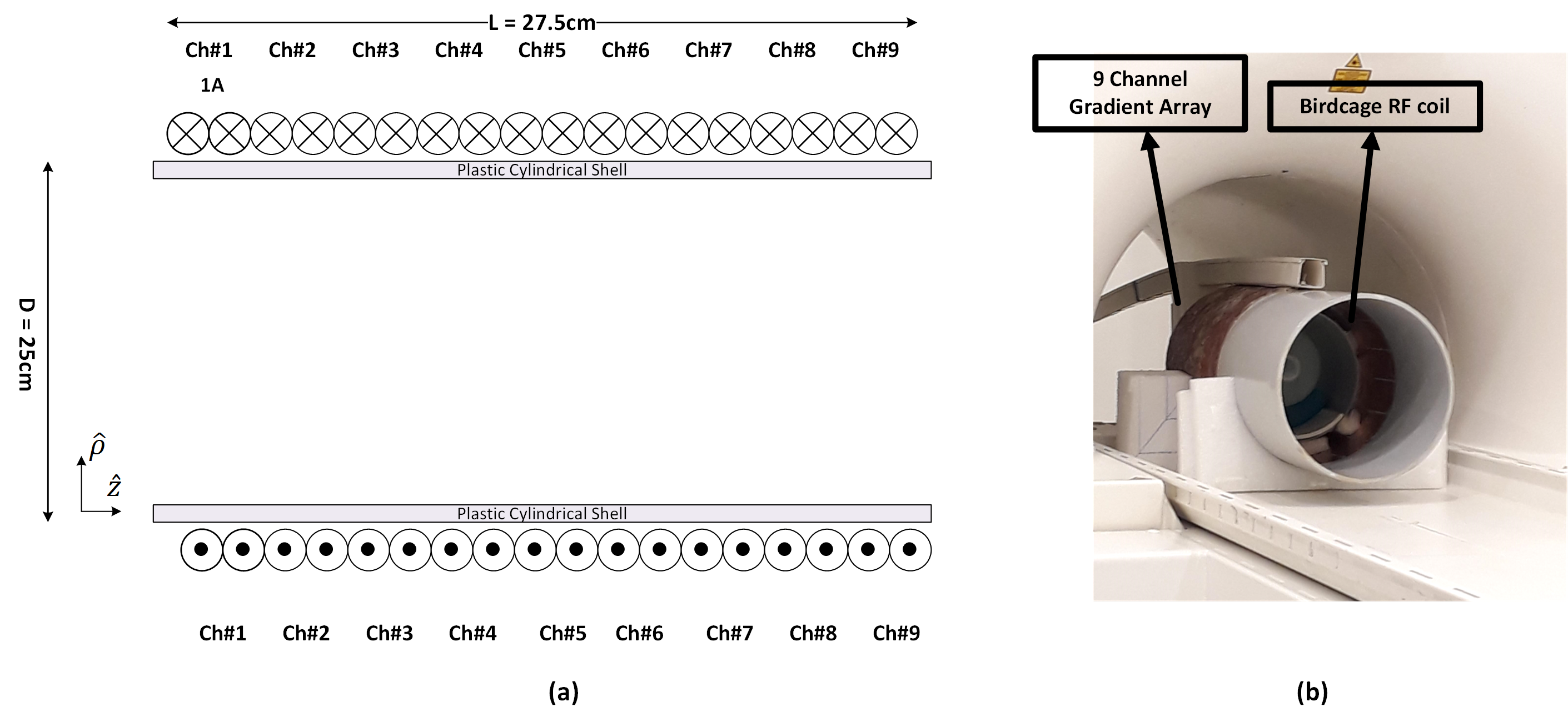
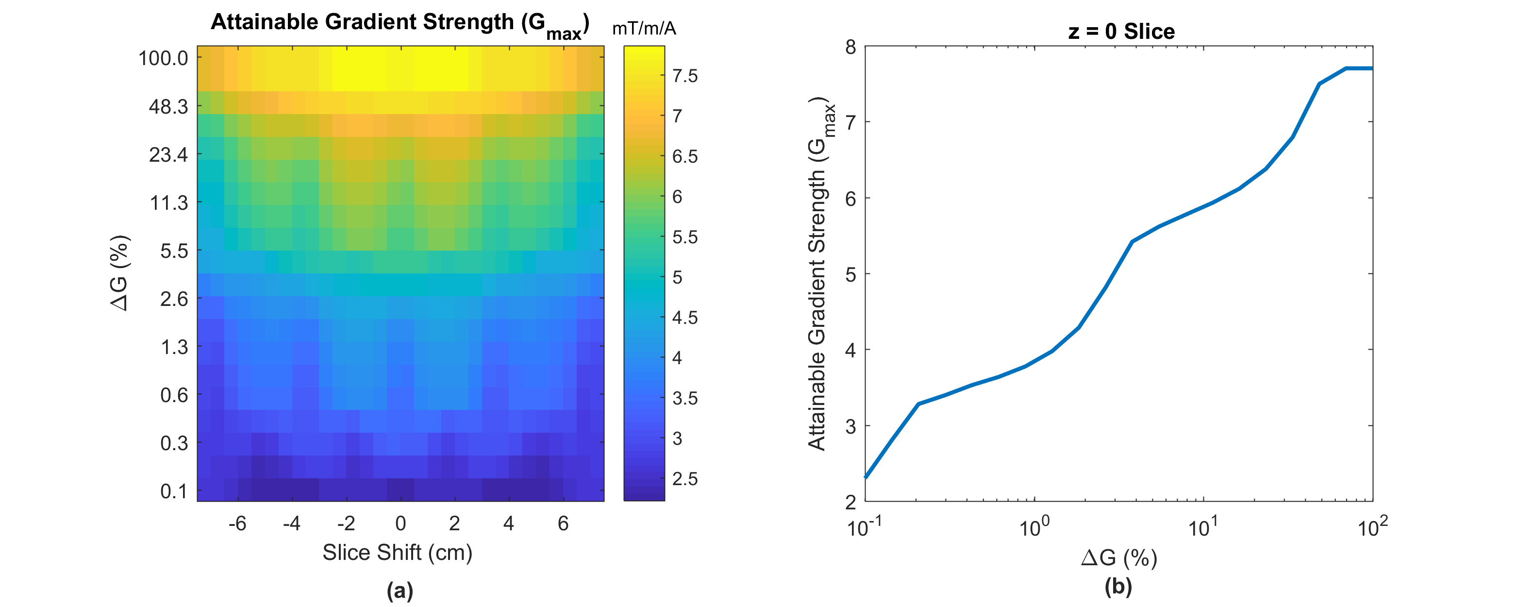
A previously designed nine channel gradient array coil2 is shown in Fig. 1. A cylindrical volume with a diameter and length of 15 cm is determined as the general VOI as an example scenario. Two types of target volumes are defined as the entire VOI (BVOI) and central slice (Bslice) in z-direction, as shown in Fig.2. A linear programming problem is formulated to solve for the optimal current weights of the array elements that maximize the gradient strength per unit current limitations of the amplifier (Gmax) for predefined peak percentage gradient linearity error (ΔG) limitations. Additionally, the effect of the ΔG inside the target slice is investigated for additional increase in the Gmax. The effect of the ΔG on the b-value can be post-corrected3. Gmax is simulated for various slice locations and ΔGs. A cylindrical homogenous phantom with a diameter of approximately 11 cm, and isotropic diffusion coefficient of 2200 µm2/s is used in the experiments. T2 of the phantom is 75 ms, which is similar to T2 of the white matter. Although our custom-designed gradient amplifiers are designed as 40V and 20A, the maximum current is chosen as 7.5A to reduce the phase errors that might occur due to mechanical vibrations and possible instability of the amplifiers. Due to low current of the amplifiers, b-values are chosen as 175 s/mm2 for both BVOI and Bslice to demonstrate the proof of principle. T2 weighted spin echo images are acquired with 100% phase oversampling and averaging factor of 4 in a 150×150 mm FOV using a 3T MRI scanner (Tim Trio, Siemens). Diffusion gradients in the z-direction are applied with the array coil and all other imaging gradients are applied with the system gradient coils.Results
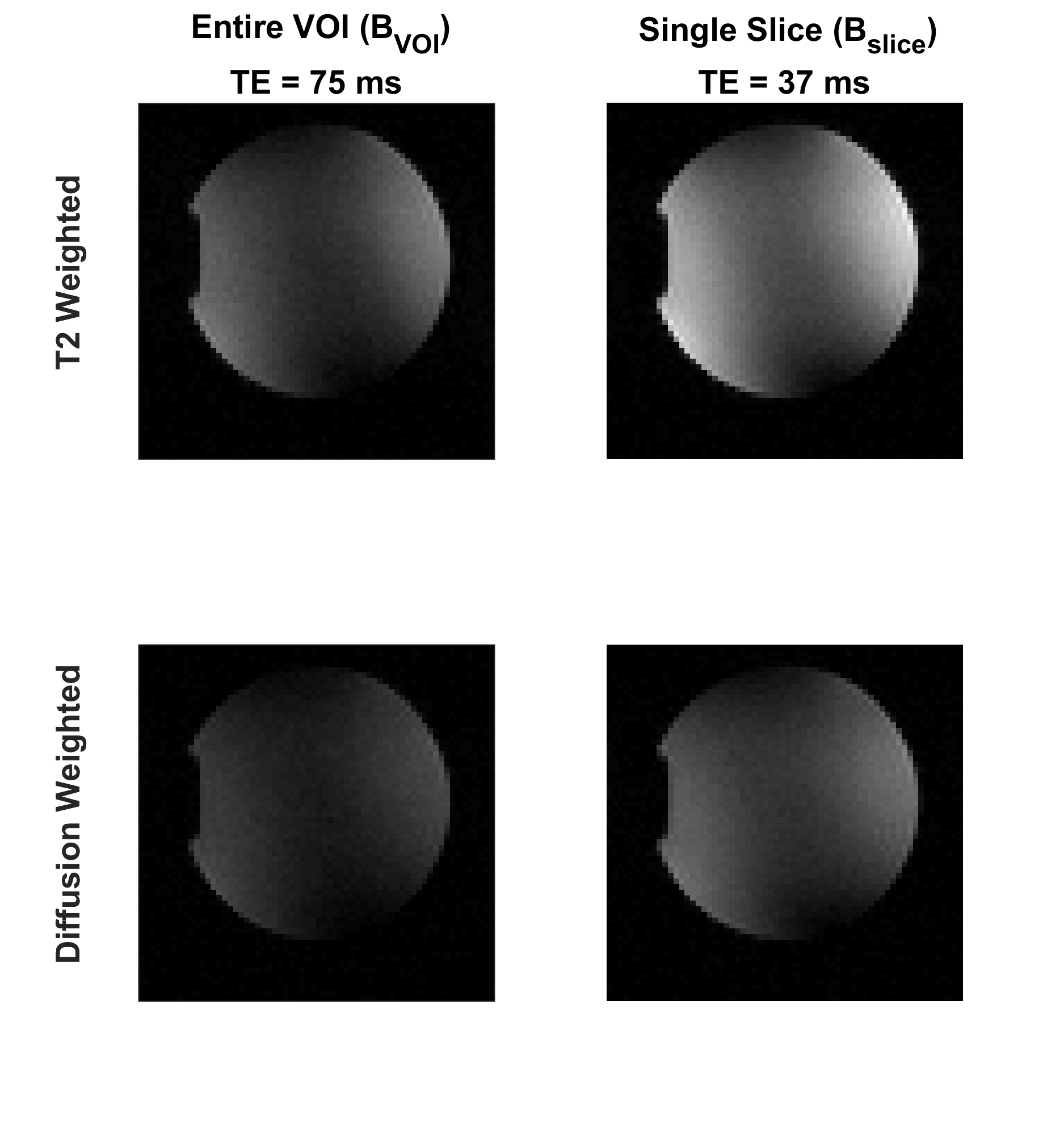
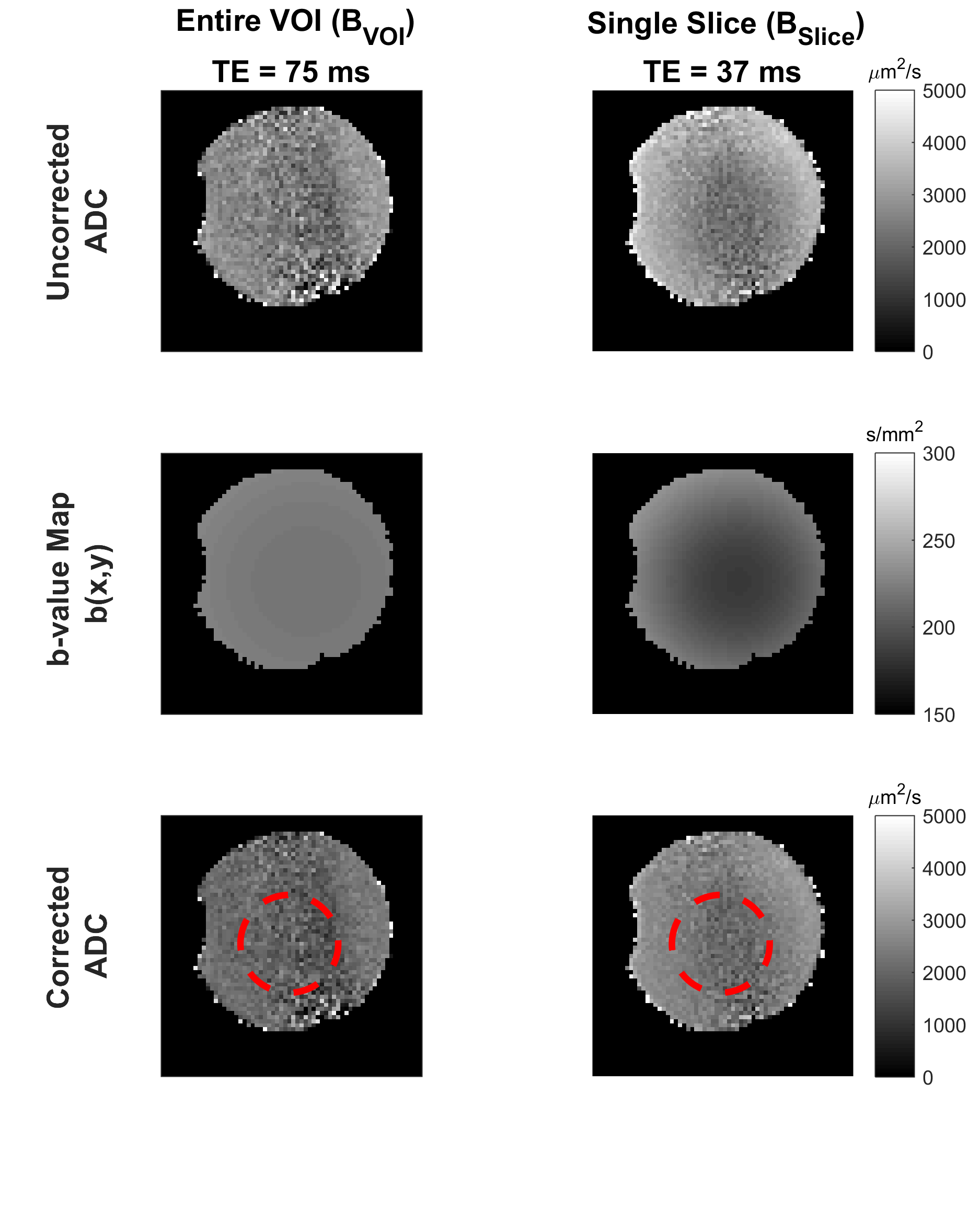
Optimized gradient field distributions for BVOI and Bslice with ΔG = 6% are shown in Fig.2. Gmax values are 1.4mT/m/A and 5.5mT/m/A for BVOI and Bslice respectively. In Fig.3, Gmax is reported for various ΔG values at every possible single slice location inside the VOI. Fig. 3 validates that slice locations can be shifted within the VOI with approximately equal Gmax. Furthermore, higher Gmax can be achieved by sacrificing field linearity. Attainable maximum gradient strength for Bslice is 4 times higher which shortened the diffusion gradients almost 3 times in our sequence timing. Figure 4 shows the diffusion weighted images acquired using BVOI (TE=75ms) and Bslice (TE=37ms). Such a TE difference causes nearly 66% increased signal level for Bslice, considering T2=75 ms for the phantom. In Figure 5, b-value is calculated at each voxel separately using current weighted superposition of the previously measured magnetic field maps2. This spatial map of b-value is used to correct the ADC maps. Inside a target region of 55mm diameter ROI, the ADC is 1900±400µm2/s for BVOI, which is lower than expected due to low SNR of BVOI4. The ADC map acquired using BSlice provides more accurate values of 2200± 300µm2/s with reduced standard deviation.Discussion and Conclusion
Preliminary experiments and simulations suggests that both local optimization of gradient fields only inside the target volume and/or more relaxed ΔG limitations provides increased Gmax, which leads to shorter diffusion durations and shorter TE. The method is validated for z-gradient due to the geometry of our windings. More generalized array of loops coils5,6 such as multi-coil or matrix coil, can be used to extend this work to arbitrary directions. Proposed method is also applicable for both whole body gradient coils and head insert gradient coils7,8 and can be used to further increase the gradient strengths in reduced target volumes.Acknowledgements
No acknowledgement found.References
[1] Setsompop K, Kimmlingen R, Eberlein E, Witzel T, Cohen-Adad J, McNab JA, Keil B, Tisdall MD, Hoecht P, Dietz P. Pushing the limits of in vivo diffusion MRI for the Human Connectome Project. Neuroimage 2013;80:220-233.
[2] Ertan K, Taraghinia S, Mohammadi H, Atalar E. Gradient Field Design for RF Excitation in Simultaneous Multi-Slice and Simultaneous Multi-Slab Imaging by Using a Z-Gradient Array. In Proceedings of the 25th Annual Meeting of ISMRM, Honolulu, Hawaii, USA, 2017. Abstract# 423]
[3] Bammer, R., Markl, M., Barnett, A., Acar, B., Alley, M.T., Pelc, N.J., Glover, G.H. and Moseley, M.E. (2003), Analysis and generalized correction of the effect of spatial gradient field distortions in diffusion-weighted imaging. Magn. Reson. Med., 50: 560–569. doi:10.1002/mrm.10545
[4] Jones, D. K. and Basser, P. J. (2004), “Squashing peanuts and smashing pumpkins”: How noise distorts diffusion-weighted MR data. Magn. Reson. Med., 52: 979–993. doi:10.1002/mrm.20283
[5] Littin, S., Jia, F., Layton, K. J., Kroboth, S., Yu, H., Hennig, J. and Zaitsev, M. (2017), Development and implementation of an 84-channel matrix gradient coil. Magn. Reson. Med.. doi:10.1002/mrm.26700
[6] Juchem C, Rudrapatna SU, Nixon TW, de Graaf RA. Dynamic multi-coil technique (DYNAMITE) shimming for echo-planar imaging of the human brain at 7 Tesla. Neuroimage 2015;105:462-472.
[7] Weiger, M., Overweg, J., Rösler, M. B., Froidevaux, R., Hennel, F., Wilm, B. J., Penn, A., Sturzenegger, U., Schuth, W., Mathlener, M., Borgo, M., Börnert, P., Leussler, C., Luechinger, R., Dietrich, B. E., Reber, J., Brunner, D. O., Schmid, T., Vionnet, L. and Pruessmann, K. P. (2017), A high-performance gradient insert for rapid and short-T2 imaging at full duty cycle. Magn. Reson. Med. doi:10.1002/mrm.26954
[8] Lee, S.-K., Mathieu, J.-B., Graziani, D., Piel, J., Budesheim, E., Fiveland, E., Hardy, C. J., Tan, E. T., Amm, B., Foo, T. K.-F., Bernstein, M. A., Huston, J., Shu, Y. and Schenck, J. F. (2016), Peripheral nerve stimulation characteristics of an asymmetric head-only gradient coil compatible with a high-channel-count receiver array. Magn. Reson. Med., 76: 1939–1950. doi:10.1002/mrm.26044
Figures