1640
Spatially Varying Signal-Drift Correction in Diffusion MRI1Department of Biomedical Engineering, The University of North Carolina at Chapel Hill, Chapel Hill, NC, United States, 2Biomedical Research Imaging Center (BRIC), The University of North Carolina at Chapel Hill, Chapel Hill, NC, United States, 3Department of Radiology, The University of North Carolina at Chapel Hill, Chapel Hill, NC, United States
Synopsis
The magnetic field in
Purpose
Diffusion MRI typically requires longer acquisition times to sufficiently cover a range of diffusion orientations and scales. The long scan time may result in noticeable temporal signal drift that may affect the estimation of diffusion parameters as well as tractography1-4. In this work, we show evidence of spatially-varying signal drift in in vivo data and show that local drift correction is more effective than global correction.
Methods
To demonstrate the effectiveness of local drift correction, we acquired multi-shell diffusion MRI data of an adult subject with 25 repetitions. In each repetition, the dataset consists of 64 diffusion-weighted images (DWIs) distributed in three shells (b=750,1500,3000 s/mm2) and 4 non-diffusion-weighted B0 images (one per 16 DWIs). Hence, there is a total of 1700 images including 100 B0 images. Corrections of motion, eddy-current distortions, and susceptibility artifacts were performed prior to drift correction. Real-valued signal with Gaussian noise was extracted using phase images5. The drift was characterized by capturing the signal variation at each voxel location across the B0 images as a function of time, which is represented discretely using image index $$$i$$$. For each voxel, we use a piecewise polynomial function $$$f(i)$$$ to model the drift. $$$f(i)$$$ minimizes$$p\sum_i(y_i-f(i))^2+(1-p)\int(\frac{d^2f}{di^2})^2di$$where $$$y_i$$$ is the signal intensity of a voxel of the $$$i$$$-th image. Temporal smoothness is controlled by $$$p$$$, which can be set from 0 (straight line) to 1 (cubic spline interpolant). In this work, we choose $$$p=1/(1+\frac{h^3}{6})$$$ where $$$h$$$ is the average spacing of data points. Drift correction is then performed using$$\widehat{y}_{ij}=y_{ij}\frac{f_i(1)}{f_j(i)}$$where $$$y_{ij}$$$ and $$$\widehat{y}_{ij}$$$ are the uncorrected and corrected intensity of voxel $$$j$$$ of the $$$i$$$-th image, respectively; $$$f_j(i)$$$ is the piecewise polynomial for correction at voxel $$$j$$$. To account for possible misalignment, spatial Gaussian smoothing was performed before drift correction. In summary, we (1) smooth the uncorrected images, (2) subtract the smoothed images from uncorrected images, obtaining the respective difference images, (3) perform signal drift correction on smoothed images, and (4) add the difference map to the drift-corrected images.
Results
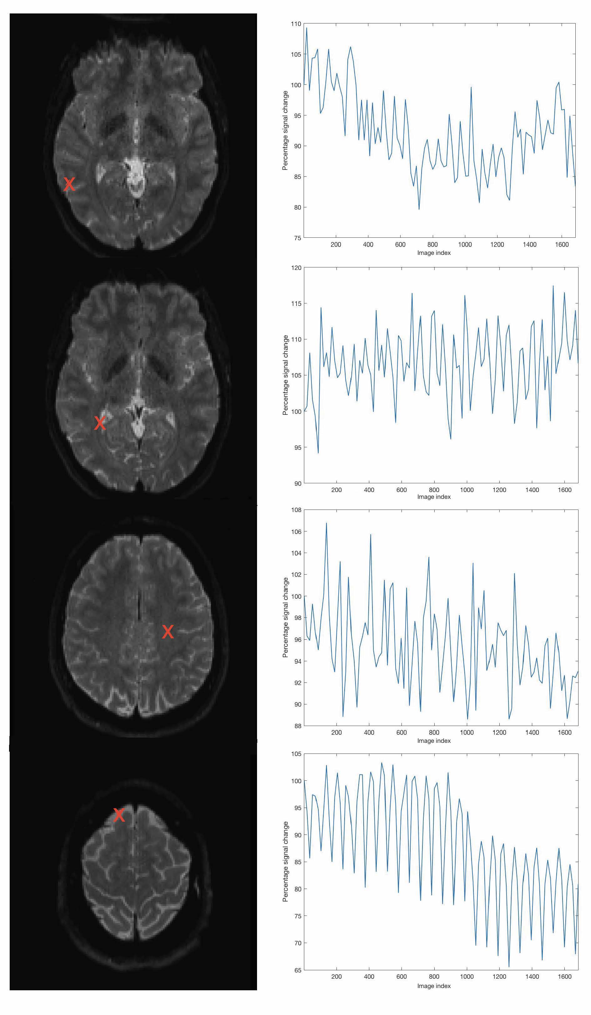
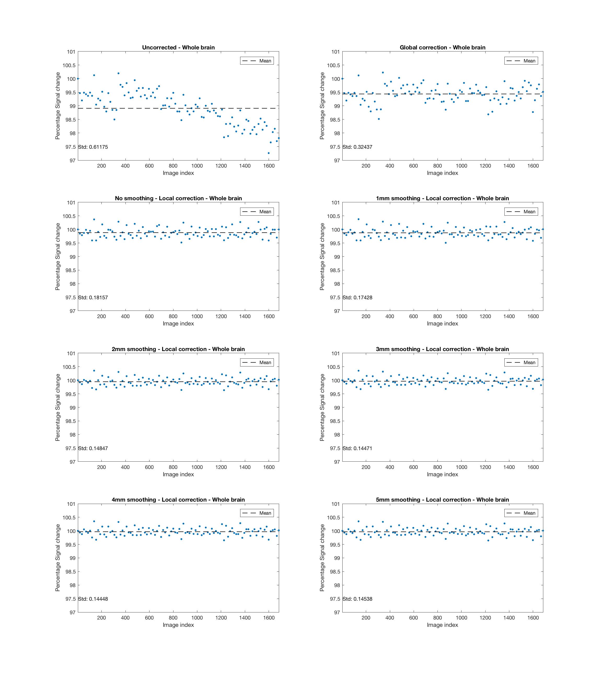
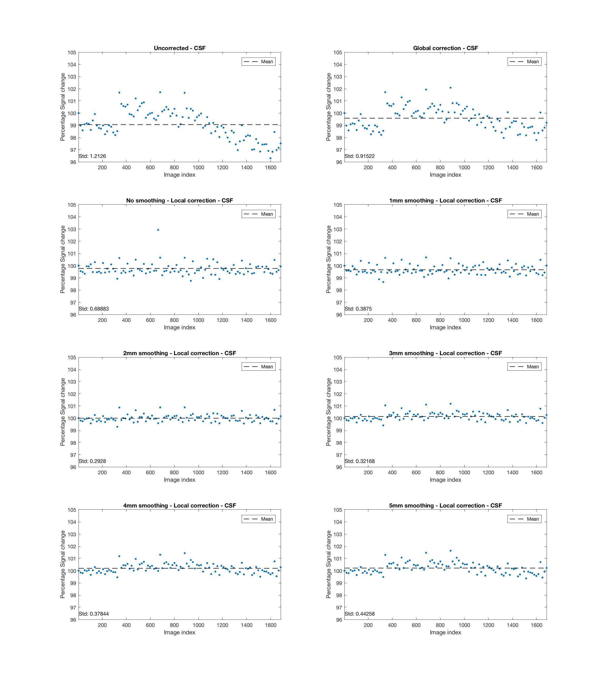
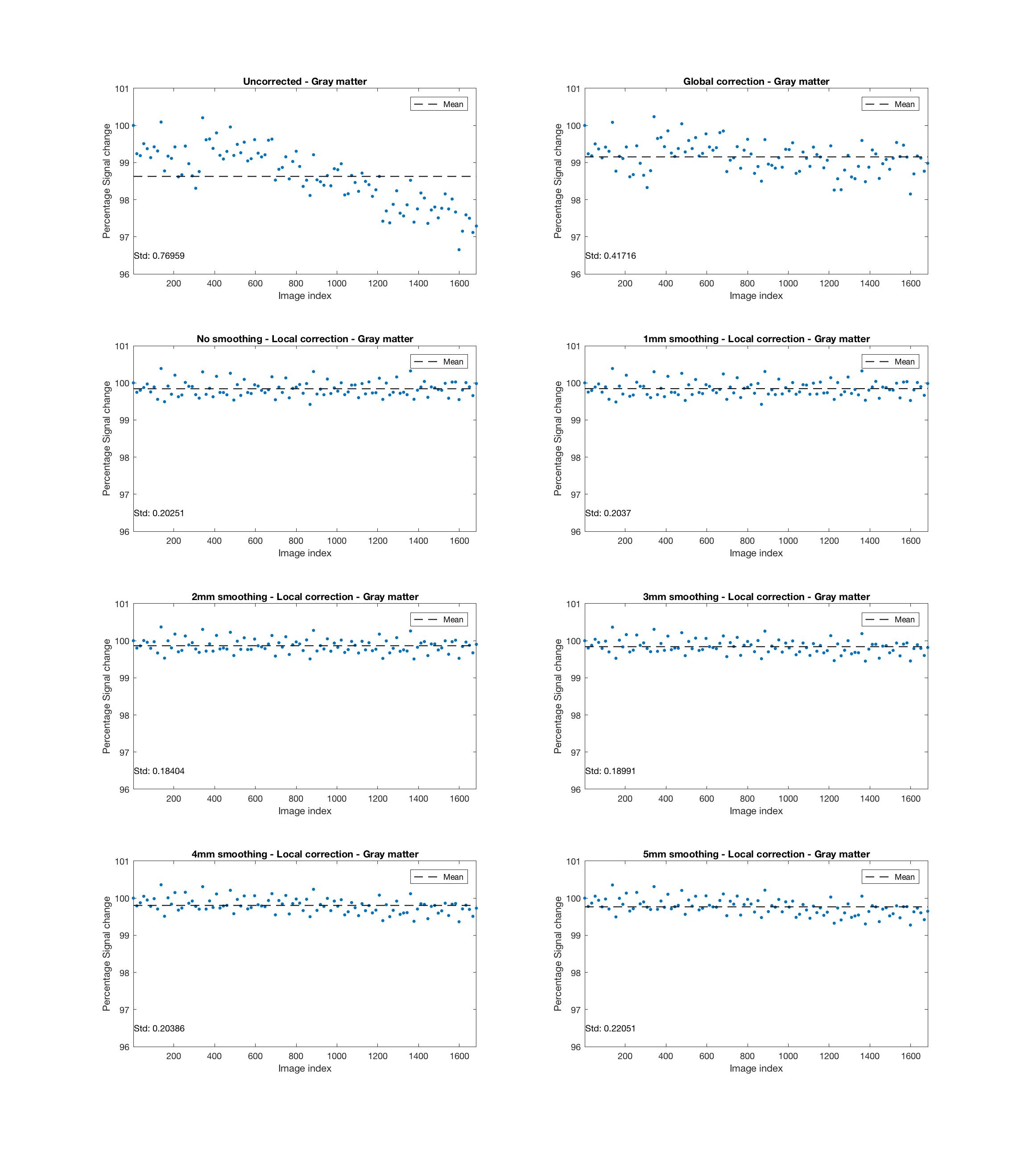
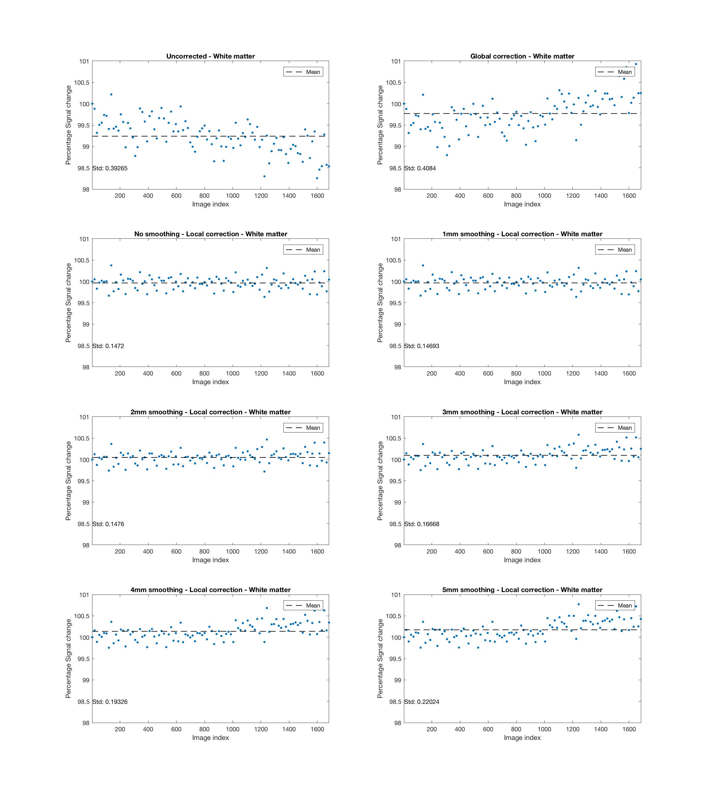
Fig. 1 shows that signal drift differs across spatial locations. Figs. 2 - 5 present results for local drift correction for varying extent of Gaussian smoothing with FWHM ranging from 0mm (no smoothing) to 5mm, in comparison with the global drift correction method introduced by Vos et al.1. From Fig. 2, one can appreciate that the whole brain mean signal intensity is more homogenous after correction, giving smaller standard deviations of percentage signal change. Similar conclusions can be drawn for different tissue types from Figs. 3 - 5. We also note that 2-3mm smoothing yields the best results.
Conclusion
We show evidence that signal drift varies spatially and can be corrected more effectively by a spatially-varying method.Acknowledgements
This work was supported in part by NIH grants (NS093842 and EB022880).References
1. Vos SB, Tax CM, Luijten PR, Ourselin S, Leemans A, Froeling M. The importance of correcting for signal drift in diffusion MRI. Magnetic resonance in medicine. 2017;77(1):285-299.
2. Benner T, van der Kouwe AJ, Kirsch JE, Sorensen AG. Real‐time RF pulse adjustment for B0 drift correction. Magnetic resonance in medicine. 2006;56(1):204-209.
3. Thesen S, Kruger G, Muller E. Absolute correction of B0 fluctuations in echo-planar imaging. Paper presented at: Proceedings of the International Society of Magnetic Resonance in Medicine2003.
4. Ericsson A, Rauschning W, Hemmingsson A. The effect of temperature on MR relaxation times and signal intensities for human tissues. Magma. 1993;1(3-4):176-184.
5. Eichner C, Cauley SF, Cohen-Adad J, et al. Real diffusion-weighted MRI enabling true signal averaging and increased diffusion contrast. Neuroimage. 2015;122:373-384.
Figures