Synopsis

In this work, we study the effect of phase errors on the quality of image reconstructions for simultaneous multi-slice (SMS) readout-segmented echo planar imaging (RS-EPI) acquisitions. We propose an iterative split slice-GRAPPA (I-SSG) algorithm to train improved kernels using estimated diffusion weighted images (DWIs) rather than baseline images. Results from stroke patients show that the proposed I-SSG algorithm produces consistently better reconstructions than the SSG algorithm in the presence of baseline phase errors.

Introduction

Readout-segmented echo planar imaging (RS-EPI) [1] combined with simultaneous multi-slice (SMS) acquisition with blipped-controlled aliasing in parallel imaging (CAIPI) [2,3] improves spatial resolution of diffusion-weighted images (DWIs) and reduces scan time for both single-shot [2] and RS-EPI [4]. Slice-GRAPPA [2] and its improved version split slice-GRAPPA (SSG) [5] are commonly used methods to de-alias SMS DWIs using kernels trained from baseline images. When applying SSG to datasets acquired from a RS-EPI sequence, we found that SSG kernels trained from baselines do not de-alias DWIs effectively due to baseline phase errors.

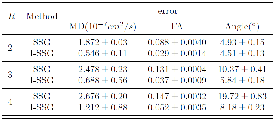
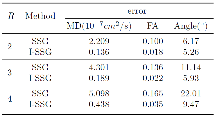
To overcome this issue, we propose an iterative approach, termed iterative split slice-GRAPPA (I-SSG), to train improved kernels using estimated DWIs rather than baseline images. Our results from a stroke patient show that proposed I-SSG produces consistently better reconstructions in the presence of baseline phase errors. It yields over 50% improvement over SSG in fractional anisotropy (FA) and mean diffusion (MD) estimations for slice reduction factors of up to R=4.

Theory and methods

We consider multi-coil and multi-slice DWIs with $$$N_c$$$ coils and $$$N_s$$$ simultaneous slices. The DWIs for the $$$i$$$-th coil, $$$l$$$-th slice, and $$$n$$$-th diffusion direction are written as

$$m_{i,l,n}(\vec{x})=|s_{l}(\vec{x})||c_{i,l}(\vec{x})|e^{j\theta_{i,l,n}(\vec{x})}a_{l,n}(\vec{x}) \quad (1)$$

where $$$\vec{x}$$$ is pixel position, $$$|s_{l}|$$$ is magnitude of baseline, $$$|c_{i,l}|$$$ is magnitude of coil sensitivity, $$$\theta_{i,l,n}$$$ is the phase, and $$$a_{l,n}$$$ is the attenuation due to diffusion.

Assume that $$$N_s$$$ phase modulated slices are acquired simultaneously according to CAIPI scheme [3] . Let superscript $$$(\phi_l)$$$ denote phase modulation of $$$l$$$-th slice. The SMS image is summation of phase modulated images, written as $$\label{eq-sms}r_{i,n} =\textstyle\sum_{l=1}^{N_s}m_{i,l,n}^{(\phi_l)}=\textstyle\sum_{l=1}^{N_s}(|s_{l}||c_{i,l}|e^{j\theta_{i,l,n}})^{(\phi_l)}a_{l,n}^{(\phi_l)} \quad (2).$$

In SSG, k-space samples of single slices are estimated by applying kernels on SMS data. The key idea of I-SSG is to use estimated DWIs, rather than baselines, to re-train kernels over time. Main steps of I-SSG are as follows. Step1. Initialization. Non-SMS baseline images are used to train initial SSG kernels. Step 2. K-space de-aliasing. Current kernels are used to de-alias SMS data in k-space and estimate single slice images $$$ \widehat{m}_{i,l,n}$$$. Step 3. Image domain de-aliasing. We estimate $$$|s_{l}||c_{i,l}|$$$ in (1) by magnitude of baseline multi-coil images without estimating coil sensitivities. Furthermore, we constrain the phase of each DWI to be the phase of SSG output from Step 2, i.e., $$$\widehat{\theta}_{i,l,n}=\measuredangle\widehat{m}_{i,l,n}$$$. From (2), we obtain the following linear system of equations.

$$\begin{bmatrix}r_{1,n} \\r_{2,n} \\\vdots \\r_{Nc,n}\end{bmatrix} =\begin{bmatrix}(|s_{1}||c_{1,1}|e^{j\widehat{\theta}_{1,1,n}})^{(\phi_l)} & \dots & (|s_{N_s}||c_{1,N_s}|e^{j\widehat{\theta}_{1,N_s,n}})^{(\phi_{N_s})}\\(|s_{1}||c_{2,1}|e^{j\widehat{\theta}_{2,1,n}})^{(\phi_1)} & \dots & (|s_{N_s}||c_{2,N_s}|e^{j\widehat{\theta}_{2,N_s,n}})^{(\phi_{N_s})} \\\vdots & \ddots & \vdots \\(|s_{1}||c_{N_c,1}|e^{j\widehat{\theta}_{N_c,1,n}})^{(\phi_1)} & \dots & (|s_{N_s}||c_{N_c,N_s}|e^{j\widehat{\theta}_{N_c,N_s,n}})^{(\phi_{N_s})}\end{bmatrix}\begin{bmatrix}\widehat{a}_{1,n}^{(\phi_1)} \\\widehat{a}_{2,n}^{(\phi_2)} \\\vdots \\\widehat{a}_{N_s,n}^{(\phi_{N_s})}\end{bmatrix} \quad (3)$$

Writing (3) in a matrix form $$$\mathbf{r}_n=\mathbf{A}_n\widehat{\mathbf{a}}_n^{(\phi)}$$$, we have

$$\label{eq-atten-est}\widehat{\mathbf{a}}_n^{(\phi)}=(\mathbf{A}_n^H\mathbf{A}_n)^{-1}\mathbf{A}_n^H\mathbf{r}_n. \quad (4)$$

Having estimated all components in (1), we update DWIs as

$$\label{dwi-est-1}\breve{m}_{i,l,n} = |s_{l}||c_{i,l}|e^{j\widehat{\theta}_{i,l,n}}\mathscr{F}^{-1}\{e^{-j\phi_l}\mathscr{F}\{\widehat{a}_{l,n}^{(\phi_l)}\}\} \quad (5)$$ where $$$\mathscr{F}\{.\}$$$ denotes 2D discrete Fourier transform.

Step 4. Tensor fitting. We combine $$$\breve{m}_{i,l,n}$$$ from (5) using sum of squares to obtain $$$\widetilde{m}_{l,n}=\sqrt{\textstyle\sum_{i=1}^{N_c}|\breve{m}_{i,l,n}|^2}$$$. The diffusion matrices are then estimated using $$\label{tensor-fitting} \widehat{D}_l,\widehat{|s_l|}=\underset{D_l,|s_l|}{\arg\min}\textstyle\sum_n||\widetilde{m}_{l,n}-|s_{l}|e^{-bg_n^TD_lg_n}||^2\text{ s.t. }D_l\succ 0, \quad (6)$$ where $$$D_l$$$ is diffusion tensor matrix, $$$g_n$$$ is $$$n$$$-th diffusion direction. Step 5. Re-train kernels. Estimates of DWIs are refined by $$\label{dwi-est-2} \check{m}_{i,l,n} = |s_{l}||c_{i,l}|e^{j\measuredangle\breve{m}_{i,l,n}}e^{-bg_n^T\widehat{D}_lg_n}. \quad (7)$$

We re-train new kernels for SSG using DWIs from (7) corresponding to diffusion direction $$$n=n_0 $$$ that has minimum mean-square-error against acquired SMS data. The tensor fitting step improves kernels by effectively de-noising estimated DWIs.

Step 6. Repeat. Go to Step 2 until algorithm converges.

Results

We used fully sampled RS-EPI data acquired from a Siemens 3T Verio scanner with 32-channel head coils. A stroke patient dataset with IRB approval and informed consent was processed. One b=0 and twenty DWIs with a b-value of 2000 s/mm² were acquired with TR=3.5 secs, TE=100 msec, 7 shots, 16 slices with slice thickness=2.1 mm, and pixel size=2.1 x 2.1 mm². Nyquist corrections, regridding, and navigator corrections were done according to [1]. SMS RS-EPI data with slice acceleration factor R=2,3,4 were simulated from pre-processed RS-EPI data by phase modulating the slices and adding them together.

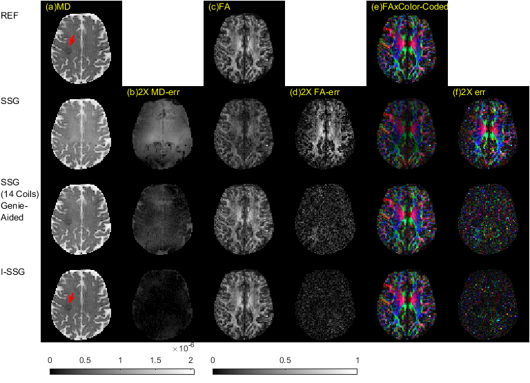
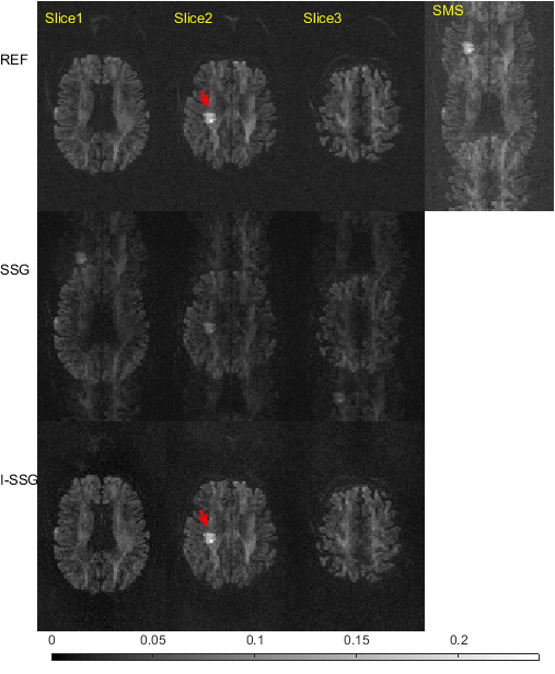
Superior performance of proposed I-SSG over SSG are shown in Table1, Table2, Fig. 1, and Fig. 2. Fig. 3 shows the convergence of I-SSG over iterations. Similar results (not shown here) were obtained for two other datasets of stroke patients.

Conclusions

Acknowledgements

References

[1] D. A. Porter and R. M. Heidemann, “High resolution diffusion-weightedimaging using readout-segmented echo-planar imaging, parallel imagingand a two-dimensional navigator-based reacquisition,” Magnetic Resonancein Medicine, vol. 62, no. 2, pp. 468–475, 2009.

[2] K. Setsompop, B. A. Gagoski, J. R. Polimeni, T. Witzel, V. J. Wedeen,and L. L. Wald, “Blipped-controlled aliasing in parallel imaging for simultaneousmultislice echo planar imaging with reduced g-factor penalty,”Magnetic Resonance in Medicine, vol. 67, no. 5, pp. 1210–1224,2012.

[3] F. A. Breuer, M. Blaimer, R. M. Heidemann, M. F. Mueller, M. A. Griswold,and P. M. Jakob, “Controlled aliasing in parallel imaging resultsin higher acceleration (caipirinha) for multi-slice imaging,” MagneticResonance in Medicine, vol. 53, no. 3, pp. 684–691, 2005.

[4] R. Frost, P. Jezzard, G. Douaud, S. Clare, D. A. Porter, and K. L. Miller,“Scan time reduction for readout-segmented epi using simultaneous multisliceacceleration: Diffusion-weighted imaging at 3 and 7 tesla,” MagneticResonance in Medicine, vol. 74, no. 1, pp. 136–149, 2015.

[5] S. F. Cauley, J. R. Polimeni, H. Bhat, L. L. Wald, and K. Setsompop,“Interslice leakage artifact reduction technique for simultaneous multisliceacquisitions,” Magnetic Resonance in Medicine, vol. 72, no. 1, pp.93–102, 2014.