Synopsis

Phase Correction is a post-processing procedure exploiting the phase of magnetic resonance images in order to obtain real-valued images containing tissue contrast with additive Gaussian noise, as opposed to magnitude images which are typically affected by a bias due to the Rician distribution of noise. This bias is particularly relevant in Diffusion Weighted Images where the signal-to-noise ratio is intrinsically low. We propose a method for automatically assessing the optimal amount of required correction based on properties of the noise affecting the images: its variance and positional non-stationarity. We present results for diffusion metrics such as FA, AD, and MD.

Introduction

Phase Correction¹ (PC) is a post-processing procedure that exploits the phase of images acquired in Magnetic Resonance Imaging (MRI) to obtain real-valued images containing tissue contrast with additive Gaussian noise, as opposed to magnitude images which are typically affected by bias due to the Rician noise distribution. This bias is particularly relevant in Diffusion Weighted Images (DWIs) where the signal-to-noise ratio (SNR) is intrinsically low².

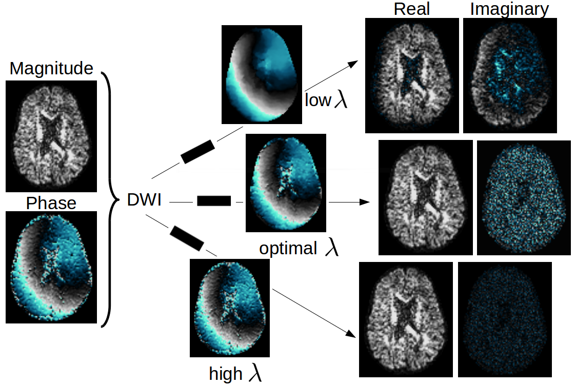
Modern PC techniques^3-5 rely on filtering each complex DWI to estimate its phase that is used to complex-rotate the image content into the real part, which is natively affected by Gaussian noise, thus bias-free. Recently,⁶ it was shown that the amount of filtering used to perform PC severely affects the outcome of the correction. Particularly, too little filtering does not produce enough bias reduction in parameters estimated, for instance, with Diffusion Tensor Imaging⁷ (DTI) - AD, RD, MD, FA⁸ - whereas too much can induce even more bias than when using magnitude DWIs.

We propose a method for automatically assessing the optimal amount of filtering that is necessary to perform PC (Fig. 1). The method produces optimally phase-corrected DWIs where the imaginary part only contains Gaussian-distributed noise. To show the results, we build on a recent technique⁴ that is based on total variation (TV) regularization, but the proposed approach is general. Secondly, we account for the noise positional non-stationarity in images due, for instance, to the multi-coil reconstruction⁹. Hence, we propose a method to estimate noise spatial variability on an acquired MRI noise map. We show synthetic results that prove the effectiveness of the proposed automatic and spatially varying PC. We also present results on data acquired with SENSE¹⁰, where magnitude DWIs are Rician-distributed⁹.

Methods

The corrected DWI at each pixel position $$$x,y$$$ is

$$DWI(x,y)^{pc} = |DWI(x,y)| e^{j \left( {\phi(x,y)} - \hat{\phi}(x,y) \right)}$$

where $$$\hat{\phi}$$$ and $$${\phi}$$$ indicate the estimated and measured phase. We propose to estimate the phase as the angle of the filtered DWI, $$$I$$$, via TV as previously reported⁴. However, our proposed version differs from the state-of-the-art for the presence of a weighting function, $$$w(x,y)$$$ that accounts for the spatial variability of noise and that scales the Lagrange multiplier $$$\lambda$$$

$$\underset{I(x,y)\in\mathbb{C}}{\operatorname{inf}} \lambda \int_{X,Y} w(x,y) [I_0(x,y)-I(x,y)]^2 dxdy + \int_{X,Y} |\nabla{I(x,y)}| dxdy$$

where $$$X,Y$$$ is the pixel domain, $$$I_0$$$ the original complex DWI.

The proposed automatic regularization fulfills the discrepancy criterion

$$\|I - I_0\|^2_2 = XY\hat{\sigma}^2$$

with $$$\hat{\sigma}^2$$$ being the estimated noise variance. The previous equation encodes the idea that the correct estimation should result in residuals described by the noise variance. We employ the following iterative law¹¹

$$\lambda_n = \lambda_{n-1} \frac{\|I-I_0\|_2}{ \sqrt{XY}\hat{\sigma}}$$

which converges to the optimal $$$\lambda$$$.

We account for spatial variability of the noise variance by setting $$$w(x,y)$$$ such that no energy is added to the above minimization problem. Therefore, we set

$$w(x,y) = \frac{{\sigma}(x,y)^2 }{ \bar{\sigma}^2 }$$

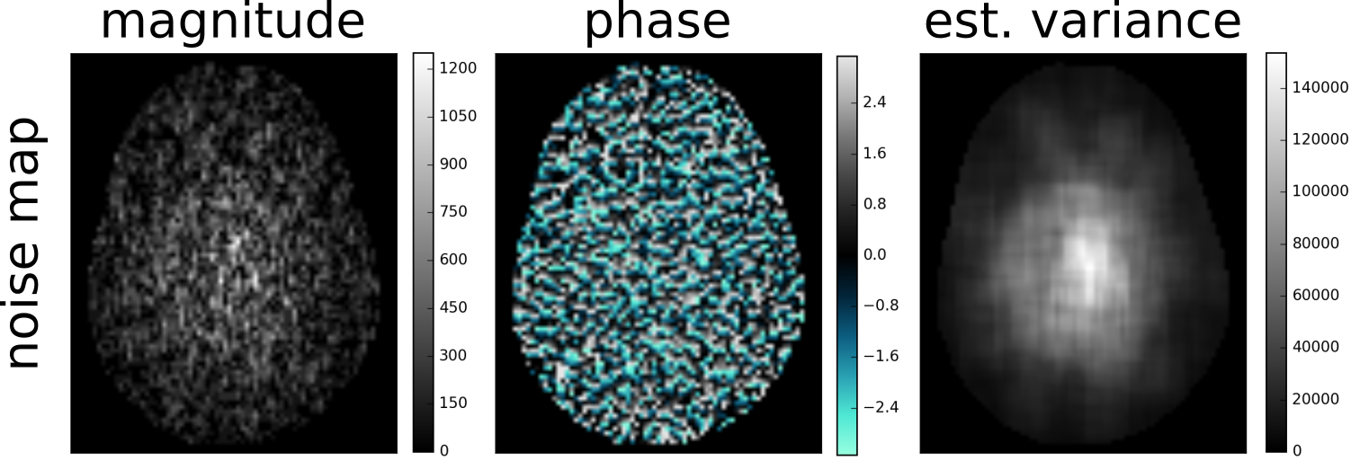
where $$$\bar{\sigma}^2$$$ is the mean variance and $$${\sigma}(x,y)^2 $$$ is the local one. We propose to estimate the local variance with a standard deviation filter of 15 pixels radius footprint on a single complex MRI noise map (Fig. 2).

Results

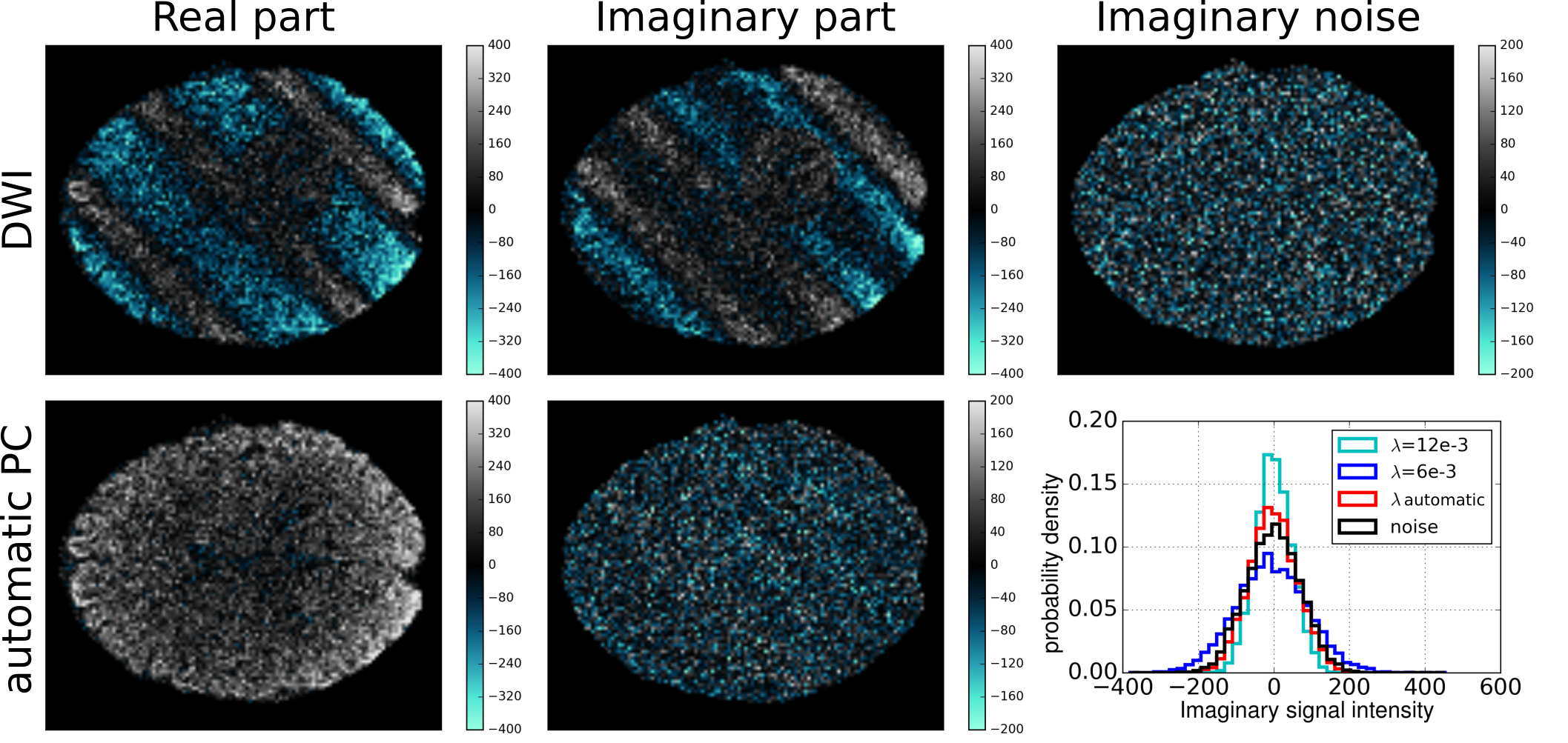
Synthetic complex DWIs were generated as previously done⁶ based on a Human Connectome Project dataset, setting $$$SNR=10$$$ and $$$b=2000\,s/mm^2$$$. These were fed to our PC algorithm.

In Fig. 3 we show the DWI before and after the proposed automatic PC, as well as the imaginary noise added to the ground-truth. The imaginary DWI after PC qualitatively looks similar to the latter. The histogram quantitatively shows that automatic PC outperforms an arbitrary choice of $$$\lambda$$$ and that the imaginary histogram corresponds to that of the noise, proving the robustness of the solution. The standard deviation estimated a posteriori as

$$\hat{\sigma}=\sqrt{\frac{\|\Im{(I)} - \Im{(I_0)}\|^2_2}{XY}}$$

corresponds to the true one: $$$\hat{\sigma}=70.88 \approx \sigma = 70.25$$$.

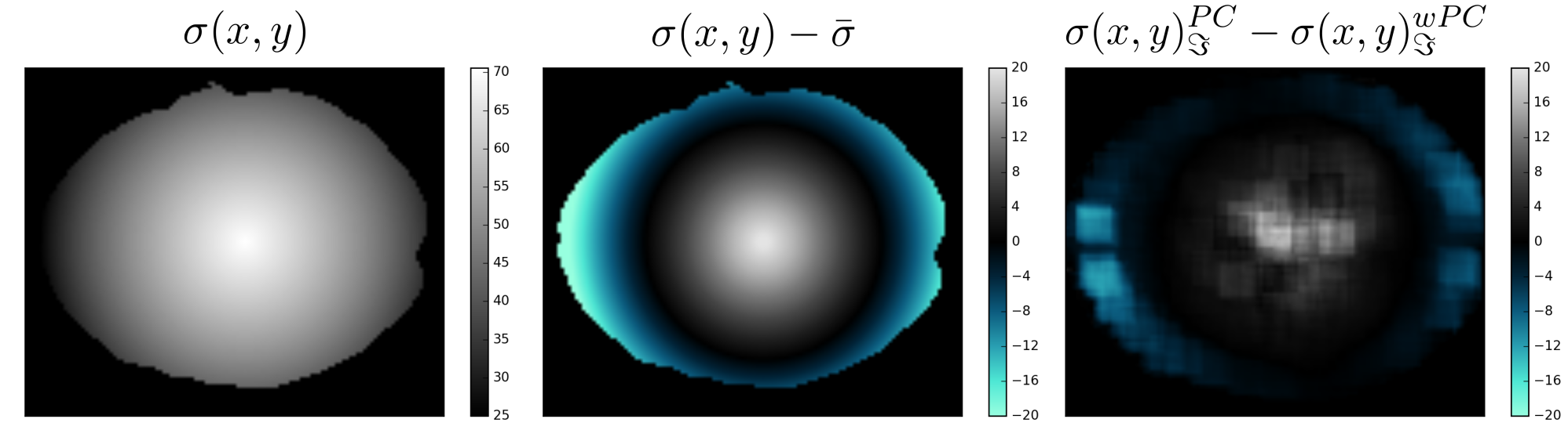
In Fig. 4 we show that spatially varying PC succeeds in accounting for noise non-stationarity. As before, the average standard deviation could be calculated a posteriori: $$$\hat{\bar{\sigma}}=51.6 \approx \bar{\sigma} = 50.46$$$.

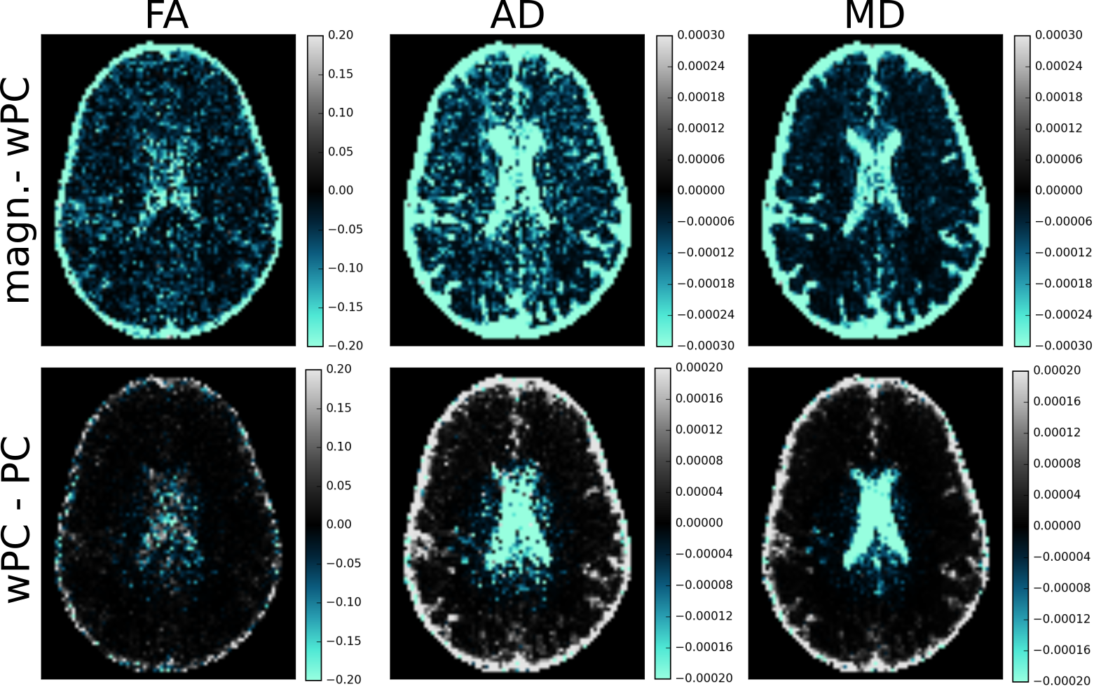
In Fig. 5-top we show quantitative differences on real data (7 directions, 7 $$$b\in{890,5562}\,s/mm^2$$$) between DTI metrics calculated on magnitude data and on automatic PC data, whereas in Fig. 5-bottom differences are related to whether spatial variability is or is not accounted for.

Discussion and conclusion

The proposed method correctly estimates the Lagrange multiplier $$$\lambda$$$ while accounting for noise spatial variability (Figs. 3,4). This resulted in important differences in vivo for DTI metrics after PC (Fig. 5). We note FA differences up to $$$20\%$$$ compared to magnitude-based results. This new PC estimates the phase effectively, removing the need of empirically choosing the correction amount, and instrumentally accounting for noise spatial variability.

Acknowledgements

Data was acquired in collaboration with the SCIL lab at the Centre de Recherche CHUS, Sherbrooke, Québec, Canada. A special thank to Maxime Descoteaux and Guillaume Gilbert for the access to the data and its preprocessing.

[For simulations,] data was provided by the Human Connectome Project, WU-Minn Consortium (Principal Investigators: David Van Essen and Kamil Ugurbil; 1U54MH091657) funded by the 16 NIH Institutes and Centers that support the NIH Blueprint for Neuroscience Research; and by the McDonnell Center for Systems Neuroscience at Washington University.

References

1. Bernstein, M.A., Thomasson, D.M., Perman, W.H., (1989) Improved detectability in low signal-to-noise ratio magnetic resonance images by means of a phase-corrected real reconstruction. Medical Physics 16, 813–817.

2. Jones, D.K., Basser, P.J., (2004) Squashing peanuts and smashing pumpkins: How noise distorts diffusion-weighted MR data. Magnetic Resonance in Medicine 52, 979–993.

3. Prah, D.E., Paulson, E.S., Nencka, A.S., Schmainda, K.M., (2010) A simple methodfor rectified noise floor suppression: Phase-corrected real data reconstruction withapplication to diffusion-weighted imaging. Magnetic resonance in medicine 64, 418–429.

4. Eichner, C., Cauley, S.F., Cohen-Adad, J., Möller, H.E., Turner, R., Setsompop, K.,Wald, L.L., (2015) Real diffusion-weighted MRI enabling true signal averaging and increased diffusion contrast. NeuroImage 122, 373–384.

5. Sprenger, T., Sperl, J.I., Fernandez, B., Haase, A., Menzel, M.I., 2016. Real valued diffusion-weighted imaging using decorrelated phase filtering. Magnetic resonance in medicine.

6. Pizzolato M., Fick R., Boutelier T., Deriche R. (2017) Noise Floor Removal via Phase Correction of Complex Diffusion-Weighted Images: Influence on DTI and q-Space Metrics. In: Fuster A., Ghosh A., Kaden E., Rathi Y., Reisert M. (eds) Computational Diffusion MRI. MICCAI 2016. Mathematics and Visualization. Springer, Cham.

7. Basser, P.J., Mattiello, J., LeBihan, D., (1994a) Estimation of the effective self-diffusion tensor from the NMR spin echo. Journal of Magnetic Resonance, Series B103, 247–254.

8. Basser, P.J., Mattiello, J., LeBihan, D., (1994b) MR diffusion tensor spectroscopy and imaging. Biophysical journal 66, 259.

9. Aja-Fernández, S., Tristán-Vega, A., (2013) A review on statistical noise models for magnetic resonance imaging. LPI, ETSI Telecomunicacion, Universidad deValladolid, Spain, Tech. Rep.

10. Pruessmann, K.P., Weiger, M., Scheidegger, M.B., Boesiger, P., et al. (1999) Sense: sensitivity encoding for fast MRI. Magnetic resonance in medicine, 42(5): 952–962.

11. Chambolle, A., (2004) An algorithm for total variation minimization and applications. Journal of Mathematical imaging and vision 20, 89–97.