1629
In vivo DTI-based free-water elimination with T2-weighting1Institute of Neuroscience and Medicine 4, Forschungszentrum Jülich, Jülich, Germany, 2Institute of Biomedical Engineering and Nanomedicine, National Health Research Institutes, Miaoli, Taiwan, 3Institute of Medical Device and Imaging, National Taiwan University College of Medicine, Taipei, Taiwan, 4Department of Neurology, Faculty of Medicine, RWTH Aachen University, Aachen, Germany, 5JARA – BRAIN – Translational Medicine, RWTH Aachen University, Aachen, Germany, 6Institute of Neuroscience and Medicine 11, Forschungszentrum Jülich, Jülich, Germany, 7Biomedical Imaging, School of Psychological Sciences, Monash University, Melbourne, Australia
Synopsis
Free-water elimination allows one to reduce the bias in DTI metrics induced by partial-volume effects. Unfortunately the fitting problem for this model is ill-conditioned. However, it has been recently demonstrated that the introduction of a second dimension determined by the echo-time, leads to a well-conditioned fitting problem. In this work we investigate the experimental design and data analysis pipeline of such experiments in vivo.
Introduction
Free-water elimination (FWE) has been proposed to reduce the
bias in DTI metrics induced by partial-volume effect (PVE).1,2 It has
been shown to be sensitive to the free-water content in the substantia nigra in
Parkinson’s patients3
and useful in detecting
microstructural white matter alterations in Alzheimer’s disease.4
Unfortunately, the fitting problem is
inherently ill-conditioned and consequently usually problematic.1,5
However, it has been recently demonstrated that the addition of a second
dimension, in this case spanned by the echo-time, TE, i.e., weighted by the transverse relaxation time, T2, transforms the problem into
a well-conditioned one.7 Thus the aim of this work is to investigate
the experimental design and data analysis workflow for FWE with T2 weighting (FWET2)
in vivo.Methods
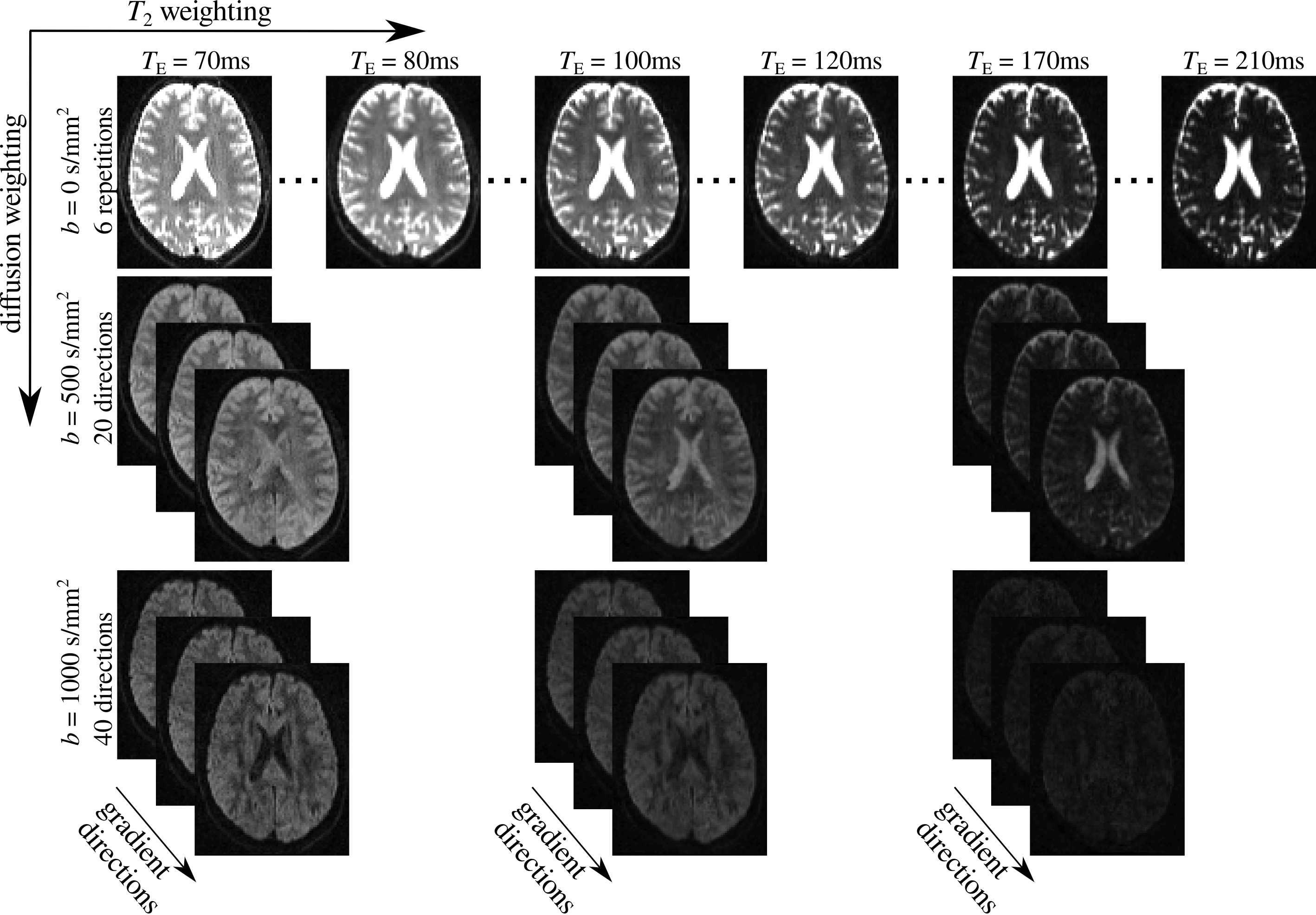
The model we adopt here assumes that the diffusion MRI signal originates from two compartments with different transverse relaxation rates and diffusivities, in the slow-exchange limit1,7 $$S\left( T_\mathrm{E},b ,\mathbf{g}\right)=S_0\left[ f_\mathrm{w}e^{-\frac{T_\mathrm{E}}{T_{2,0}}}e^{-bD_0}+\left(1-f_\mathrm{w}\right)e^{-\frac{T_\mathrm{E}}{T_{2,\mathrm{t}}}}e^{-b\mathbf{g}^\mathrm{T}\mathbf{D}\mathbf{g}}\right]\mathrm{, (1)}$$ where S0 is the proton density, fw, T2,0 and D0 are the fraction, transverse relaxation time and diffusion coefficient of the free-water compartment and T2,t and D are the transverse relaxation time diffusion tensor for the tissue compartment. The experimentally controlled parameters are the strength and direction of the diffusion weighting gradient, b and g, and TE (Fig.1).
Experiments were performed on a healthy volunteer, in a 3T Siemens Trio scanner (Siemens, Erlangen, Germany). Prior written, informed consent was obtained from the volunteer. A Stejskal-Tanner pulse sequence with monopolar pulse field gradients and EPI readout was implemented for this purpose. The sequence was designed to independently control the gradient pulse duration, δ, and separation, Δ, as well as TE. Thus, the diffusion-dimension and the relaxation-dimension are fully decoupled. Experimental parameters included (Fig. 1): 4 experiments with TE = 70, 100, 130, 170 ms; b-values = 0 (6 repetitions), 500 (20 directions), 1000 (40 directions) s/mm2; Δ = 34 ms and δ = 19 ms. Additionally, we acquired 8 more echo-times, in the range TE $$$\in$$$ [70, 210] ms. The experiment with TE = 70 ms was acquired twice with opposite phase-encoding (anterior-posterior, posterior-anterior) in order to correct for EPI distortions. Other parameters were voxel-size = 23 mm3; matrix-size = 100×100×60; repetition-time, TR = 15 s and GRAPPA acceleration factor = 2.
Eddy current and EPI distortions were corrected using the EDDY toolkit available in FSL.8 FWET2 DTI parameter estimation was performed in three steps:
- Experimental data with b = 0 s/mm2 was used to generate an initial guess for T2,t using the linear least-squares (LLS) method: $$$\hat{\gamma}_\mathrm{SE}=\left(W^{\mathrm{T}}_{\mathrm{SE}}W_\mathrm{SE}\right)^{-1}W^{\mathrm{T}}_{\mathrm{SE}}y$$$, where $$$W_{\mathrm{SE}}=\left[1,-T_\mathrm{E}\right]^\mathrm{T}$$$, $$$\gamma_{\mathrm{SE}}=\left[\ln{S^\mathrm{SE}_0},1/T_{2,\mathrm{t}}\right]^\mathrm{T}$$$ and y is the measured data. Similarly the initial guess for D was generated using the DWI experiment with TE = 70 ms using LLS: $$$ \hat{\gamma}_\mathrm{DTI}=\left(W^\mathrm{T}_\mathrm{DTI}W_\mathrm{DTI}\right)^{-1}W^{\mathrm{T}}_{\mathrm{DTI}}y$$$, where $$$W_{\mathrm{DTI}}=\left[1,-bg^2_x,-2bg_xg_y,-2bg_xg_z,-bg^2_y,-2bg_yg_z,-bg^2_z,\right]^\mathrm{T}$$$ and $$$\gamma_{\mathrm{DTI}}=\left[\ln{S^\mathrm{DTI}_0},D_{11},D_{12}...,D_{33}\right]^\mathrm{T}$$$.
- Having had the initial guess for D and T2,t, an initial guess for fw was generated using the method proposed by Hoy et al.5 and Neto Henriques et al.6 using a non-linear least-squares (NLLS) method.
- Finally FWET2 was fitted via NLLS minimisation using the initial guess generated in the former steps, with the help of the Levenberg-Marquardt algorithm with in-house Matlab scripts. The power images method9 was used to reduce the bias due to background noise prior fitting. Values for D0 = 3×10⁻³ mm2/s and T2,0 = 500 ms were fixed according to literature values.10 Thus, the model parameters are $$$\gamma_\mathrm{FWET2}=\left[S_0,f_\mathrm{w},D_{11},D_{12},...,D_{33},T_{2,\mathrm{t}}\right]$$$. The NLLS estimator is given by $$\gamma_\mathrm{FWET2}=\arg \min \sum_{i} \left[y_i-S\left(T_{\mathrm{E},i},b_i,\mathbf{g}_i\right)\right]^2\mathrm{. (2)}$$
Results and Discussions
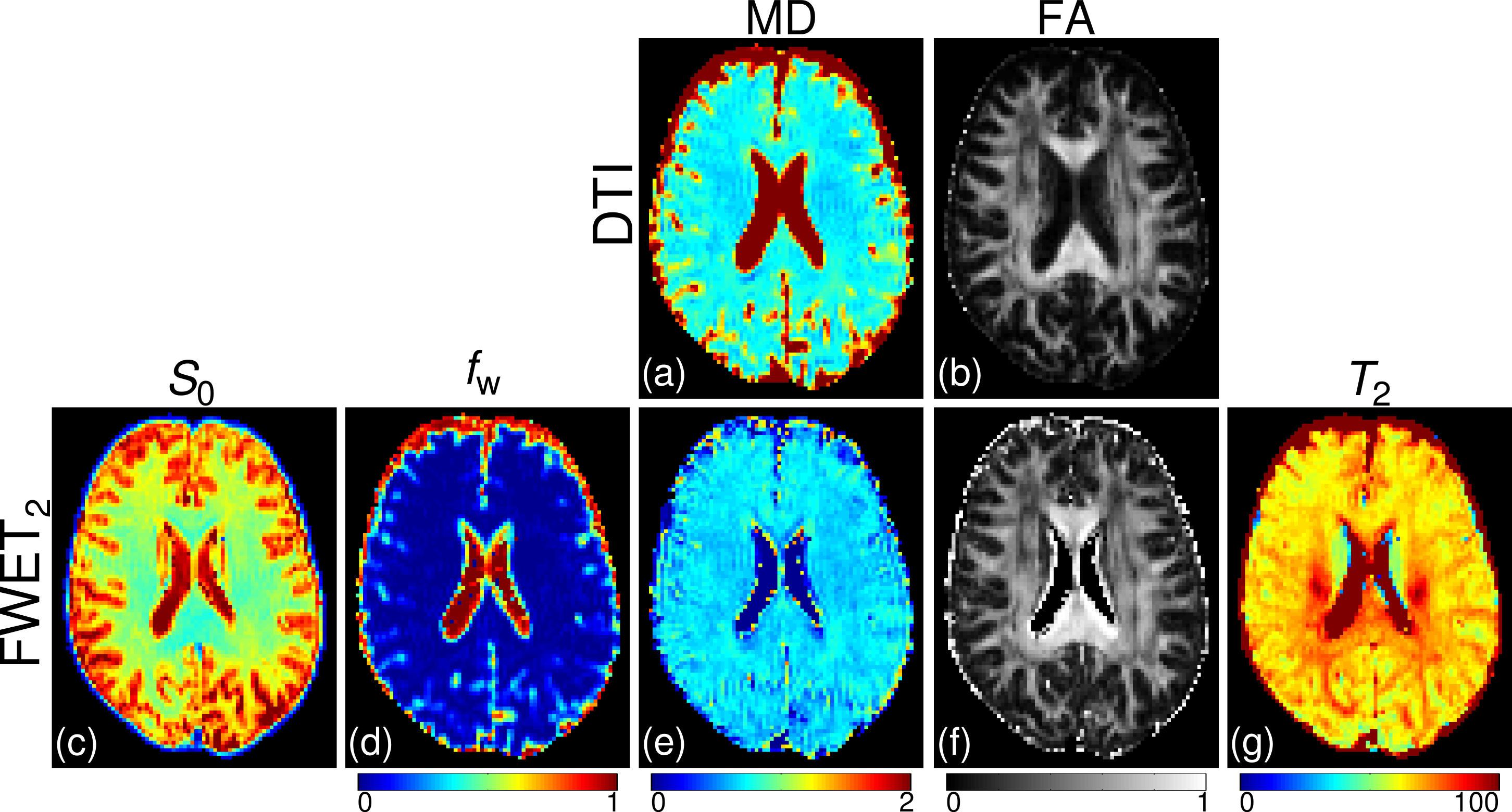
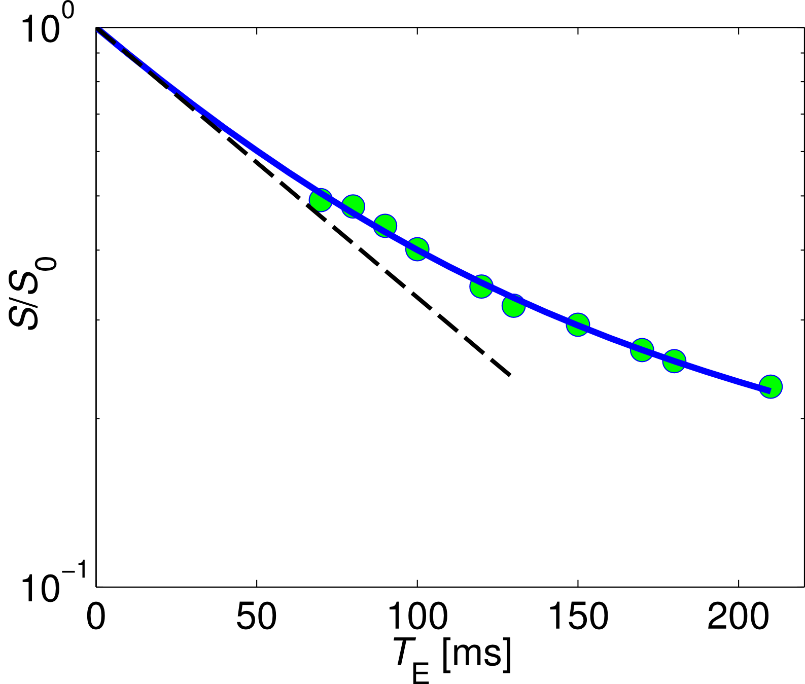
Figs. 2a and 2b show the maps of mean diffusivity (MD) and fractional anisotropy (FA) obtained with conventional DTI analysis. Figures 2c-2g exhibit the maps of S0, fw, MD, FA, and T2,t obtained via FWET2 analysis. One can observe that MD and FA from DTI show strong bias due to PVE, which is improved by using FWET2. In addition, T2,t values are in the range published in the literature.11 Figure 3 shows the only T2-weighted signal averaged over 20 voxels in the inter-hemisphere space, where fw was between 0.25 and 0.35. The solid line shows the fitting of Eq. (1). A monoexponential attenuation function is shown for reference. The signal attenuation is found to be indeed deviated from the monoexponential behaviour.Conclusions
We have successfully implemented the experimental and data analysis workflow for the FWET2 method. This allows one to reduce the bias conventional DTI metrics due to the presence of a water pool with free, isotropic diffusivity. FWET2 is particularly useful in the regions strongly affected by PVE.Acknowledgements
No acknowledgement found.References
[1] Pasternak O, et al. Free Water Elimination and Mapping from Diffusion MRI. Magn Reson Med 2009;62:717-730.
[2] Pasternak O, et al. Estimation of Extracellular Volume from Regularized Multi-Shell Diffusion MRI. Med Image Comput Comput Assist Interv 2012;15:305-312.
[3] Ofori E, et al. Increased free-water in the substantia nigra of Parkinson’s disease: a single-site and multi-site study. Neurobiol Aging 2015;36(2):1097-1104.
[4] Hoy AR, et al. Microstructural white matter alterations in preclinical Alzheimer's disease detected using free water elimination diffusion tensor imaging. PLoS One 2017;14;12(3):e0173982.
[5] Hoy AR, et al. Optimization of a free water elimination two-compartment model for diffusion tensor imaging. Neuroimage 2014;103:323-333.
[6] Neto Henriques R, et al. Exploring the potentials and limitations of improved free-water elimination DTI techniques. Proc Intl Soc Magn Reson Med 2017;1787.
[7] Collier Q, et al. Solving the free water elimination estimation problem by incorporating T2 relaxation properties. Proc Intl Soc Magn Reson Med 2017;1783.
[8] Jesper L, et al. An integrated approach to correction for off-resonance effects and subject movement in diffusion MR imaging. NeuroImage 2016;125:1063-1078.
[9] Miller AJ, Joseph PM. The use of power images to perform quantitative analysis on low SNR MR images. Magn Reson Imaging 1993;11(7):1051-6.
[10] Piechniket SK, Functional Changes in CSF Volume Estimated Using Measurement of Water T2 Relaxation. Magn Reson Med 2009;61:579-586.
[11] Gras V, et al. Diffusion-Weighted DESS Protocol Optimization for Simultaneous Mapping of the Mean Diffusivity, Proton Density and Relaxation Times at 3 Tesla. Magn Reson Med 2017;78:130-141.
Figures