1628
DTI-based free-water elimination with T2-weighting using dedicated anisotropic diffusion fibre phantoms1Institute of Neuroscience and Medicine 4, Forschungszentrum Jülich, Jülich, Germany, 2Institute of Biomedical Engineering and Nanomedicine, National Health Research Institutes, Miaoli, Taiwan, 3Department of Neurology, Faculty of Medicine, RWTH Aachen University, Aachen, Germany, 4JARA – BRAIN – Translational Medicine, RWTH Aachen University, Aachen, Germany, 5Institute of Neuroscience and Medicine 11, Forschungszentrum Jülich, Jülich, Germany, 6Biomedical Imaging, School of Psychological Sciences, Monash University, Melbourne, Australia, 7Institute of Medical Device and Imaging, National Taiwan University College of Medicine, Taipei, Taiwan
Synopsis
In this work we demonstrate the use of two dedicated anisotropic diffusion fibre phantoms for the study of free-water elimination DTI. In particular, we make use of the recently proposed approach in which an extra dimension to the diffusion weighting, namely transverse relaxation weighting, is added to the model.
Introduction
Omission of a free-water compartment in diffusion models can
potentially lead to bias in estimated parameters, especially in the case of
partial-volume effect (PVE)1-3 or tissue condition such as oedema.1 The free-water
elimination (FWE) method has been proposed to reduce such bias in DTI metrics.1-3
Inherently, the fitting problem is ill-conditioned and consequently problematic.1-5
However, it has been recently demonstrated that the addition of a transverse relaxation
weighting term to each of the compartments, transforms the problem into well-conditioned
one.5 The aim of this work is to introduce the design of two
artificial, anisotropic diffusion fibre phantoms, and to demonstrate their usability
for the study of FWE with T2
weighting (FWET2).Methods
Model. The model assumes that the diffusion MRI signal originates from two compartments with different transverse relaxation times and diffusivities1,3,5 $$S\left( T_\mathrm{E},b ,\mathbf{g}\right)=S_0\left[ f_\mathrm{w}e^{-\frac{T_\mathrm{E}}{T_{2,0}}}e^{-bD_0}+\left(1-f_\mathrm{w}\right)e^{-\frac{T_\mathrm{E}}{T_{2,\mathrm{t}}}}e^{-b\mathbf{g}^\mathrm{T}\mathbf{D}\mathbf{g}}\right]\mathrm{, (1)}$$ where S0 is the proton density, fw, T2,0 and D0 are the fraction, transverse relaxation time and diffusion coefficient of the free-water compartment, respectively. T2,t and D denote the transverse relaxation time and diffusion tensor for the tissue compartment. The experimental parameters are the strength and direction of the diffusion weighting gradient, b and g, and the echo-time, TE.
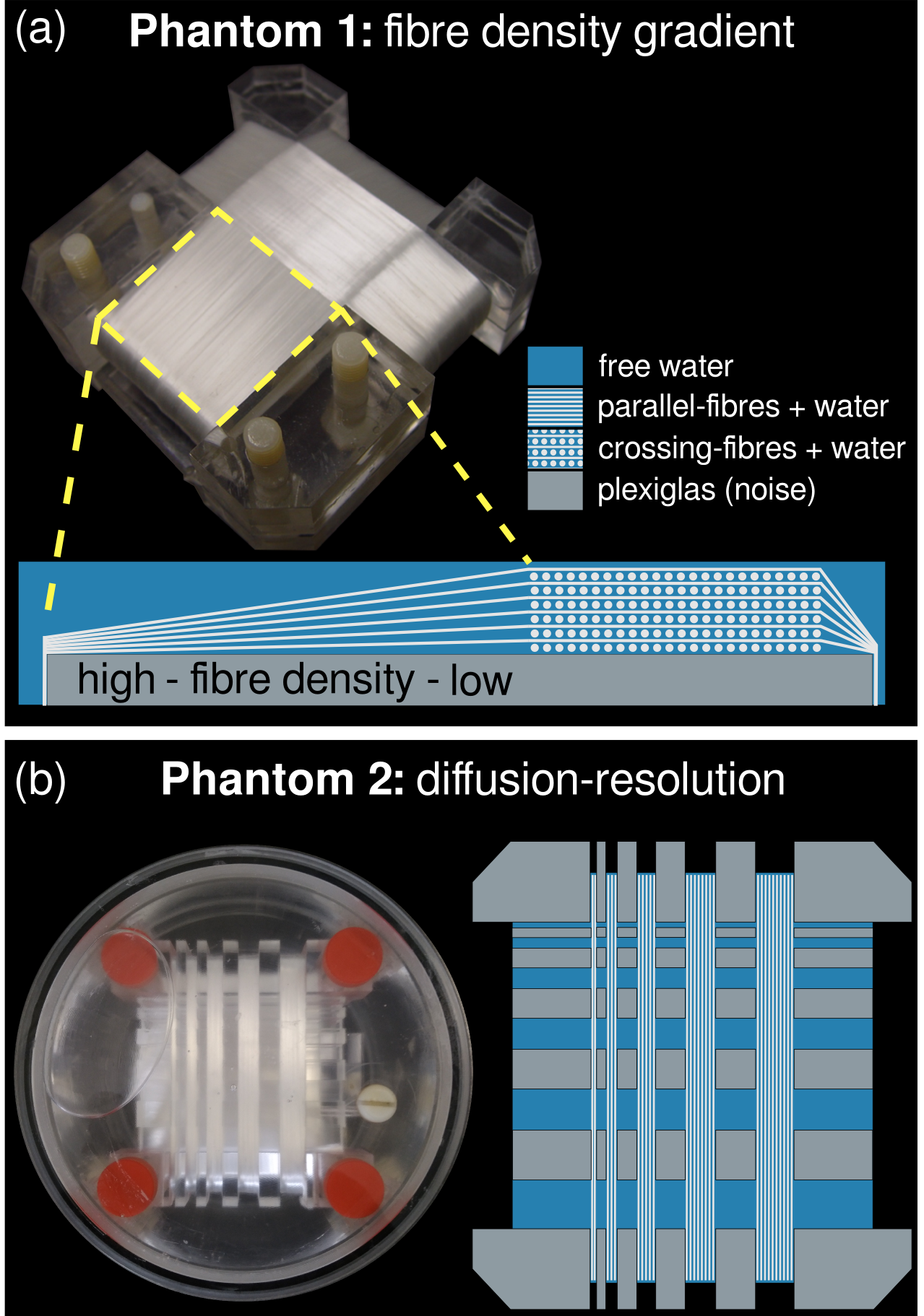
Phantoms. Both phantoms were constructed using polyethylene fibres (~8 μm in radius) wound on Perspex platforms, and submerged in a container with distilled water (Fig. 1).6,7
- Phantom 1. Multi-section phantom including a section of parallel fibres with increasing packing density, which, in turn, generates an interstitial space of decreasing size.6
- Phantom 2. Contains fibre bundles and free-water compartments of different sizes. The usefulness of this phantom lies in the investigation of PVE.
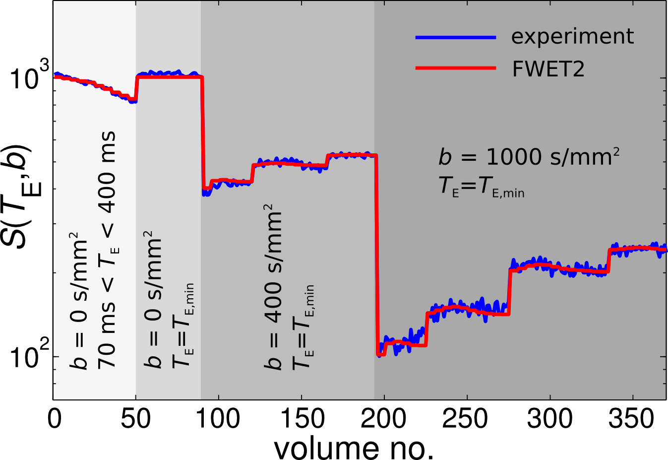
Experiments and data analysis. Measurements were performed on a 3T Siemens Prisma scanner (Siemens, Germany). A diffusion-weighted double-echo sequence with bipolar pulsed-field gradients was used. Experimental parameters included (Fig. 2): for the T2-dimension, 10 measurements with TE in the range TE $$$\in$$$ [70,400] ms, b-value = 0 s/mm2, 5 repetitions per TE. For the diffusion-dimension, b-values = 0 (8 repetitions), 400 (21 directions) and 1000 (35 directions) s/mm2; 5 repetitions. Other parameters were voxel-size = 23 mm3; matrix-size = 96×96×50; GRAPPA acceleration factor = 2.
FWET2 parameter estimation was performed in three steps with in-house Matlab scripts:
- Data with b = 0 s/mm2 was used to generate an initial estimation for T2,t using the linear least-squares estimator. Similarly, the diffusion experiment was used to generate the initial estimation for D. D0 = 2.3×10⁻³ mm2/s and T2,0 = 2.5 s were estimated in a ROI in the bulk water.
- Afterwards an initial estimation for fw was calculated following the method proposed in the works by Hoy et al.3 and Neto Henriques et al.4
- FWET2 was fitted using the initial estimations from the former steps, with the help of the Levenberg-Marquardt algorithm with in-house Matlab scripts.
Results and discussions
Fig. 2 shows the signal attenuation in the fibre area for 70 ms ≤ TE ≤ 400 ms and b = 0 s/mm2 (volumes 0-50) diffusion-attenuated signal (volumes 51-370) for b = 0, 400, 1000 s/mm2 (blue line). The red line depicts the fits of Eq. (1) to the experimental data.
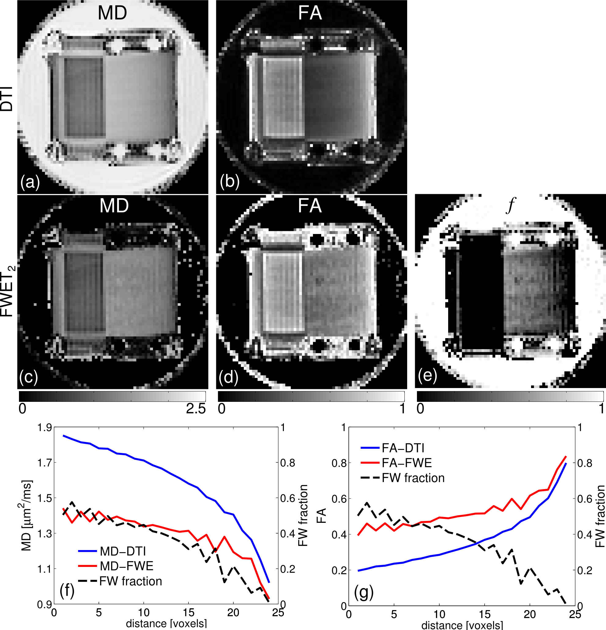
Fig. 3 summarises the results for Phantom 1. Mean diffusivity (MD) and fractional anisotropy (FA) from conventional DTI were evaluated for comparison (Fig. 3a-b). MD, FA and fw from FWET2 are shown in Fig. 3c-e. It was found that fw decreases from left to right, according to the increase in FD which is observed in the profiles shown in Figs. 3f-g.
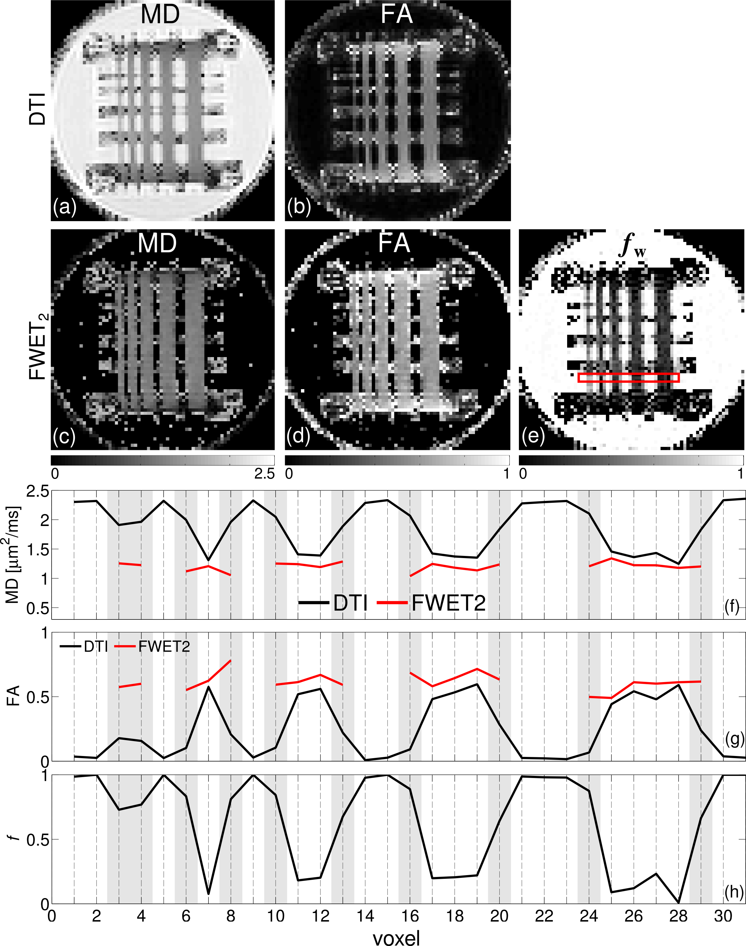
Fig. 4 summarises the results for Phantom 2. MD and FA from conventional DTI are shown in Fig. 3a-b for comparison. MD, FA and fw from FWET2 are shown in Fig. 3c-e. The thinnest fibre bundle (leftmost) appears blurred in DTI metrics, whereas it is fully recovered in FWET2 maps. This is shown in the profiles in Figs. 3f-h, taken along the ROI depicted by the red line in Fig. 4e. Grey zones represent voxels affected by PVE. It is clearly shown that FWET2 eliminates the bias observed in conventional DTI metrics.
Conclusions
We have demonstrated the application of two artificial, anisotropic diffusion fibre phantoms in the investigation of the FWET2 model. Important features, such as PVE and changes in the size of the interstitial space were successfully captured by the FWET2 model parameters.Acknowledgements
No acknowledgement found.References
[1] Pasternak O, et al. Free Water Elimination and Mapping from Diffusion MRI. Magn Reson Med 2009;62:717-730.
[2] Pasternak O, et al. Estimation of Extracellular Volume from Regularized Multi-Shell Diffusion MRI. Med Image Comput Comput Assist Interv 2012;15:305-312.
[3] Hoy AR, et al. Optimization of a free water elimination two-compartment model for diffusion tensor imaging. Neuroimage 2014;103:323-333.
[4] Neto Henriques R, et al. Exploring the potentials and limitations of improved free-water elimination DTI techniques. Proc Intl Soc Magn Reson Med 2017;1787.
[5] Collier Q, et al. Solving the free water elimination estimation problem by incorporating T2 relaxation properties. Proc Intl Soc Magn Reson Med 2017;1783.
[6] Farrher E, et al. Novel multisection design of anisotropic diffusion phantoms. Magn Reson Imaging 2012;30:518-526.
[7] Grinberg F, et al. Complex patterns of non-Gaussian diffusion in artificial anisotropic tissue models. Microporous Mesoporous Mater 2013;178:44-47.
Figures