Synopsis

IVIM parameter estimation restricted to D and f (avoiding D*) has gained increased popularity. In this study we show that the commonly used segmented fitting approach is preferable. We also show that differentiation between tumor and healthy liver tissue is substantially enhanced by the combined use of D and f.

Introduction

The intravoxel incoherent motion (IVIM) model enables extraction of diffusion and perfusion information from diffusion-weighted images¹, information important for tumor tissue characterization².

The IVIM model describes the diffusion-weighted MR signal as:

$$S=S_0\left((1-f)e^{-bD}+fe^{-bD^*}\right) \quad (1)$$

where D is the diffusion coefficient, and f and D* are related to perfusion¹. Analysis excluding D* has been used in several studies recently^3–5. Both diffusion and perfusion information can still be extracted, but with reduced scan time and requirements on e.g. signal-to-noise ratio.

Two categories of estimation approaches for D and f have been proposed. 1) A monoexponential model fit of:

$$S=S_0(1-f)e^{-bD}=Ae^{-bD} \quad (2)$$

omitting b-values below a certain threshold b_thr with f calculated as f=1–A/S(0), where S(0) is the measured signal at b=0^6–8. 2) A simplified version of the IVIM model (sIVIM) valid for {b:b=0 or b≥b_thr}:

$$S=S_0\left((1-f)e^{-bD}+f\delta(b)\right) \quad (3)$$

where $$$\delta(b)$$$ is the discrete delta function^7,9,10. Using this model, D and f can be estimated through e.g. least squares fitting. However, as for the complete IVIM model, a Bayesian approach may also be useful^8,11,12.

The aims of this study were 1) to investigate the impact of estimation approach on IVIM parameters D and f using simulated and in vivo data, and 2) to study the ability for differentiation between tumor and healthy liver tissue based on D and f.

Methods

A protocol for estimation of IVIM parameters D and f including five b-values (0,120,350,575,800s/mm²) was employed in this study.

Simulated data was generated based on the sIVIM model (Eq. 3) with Rician noise using the b-values above, and D and f in the ranges [0.5;1.5]µm²/ms and [0;0.3] respectively. Three SNR levels were studied: 10, 20 and 40, referring to SNR in the image without diffusion weighting, i.e. b=0.

Nine patients with liver metastases from neuroendocrine tumors were included in this study. They were treated with either hepatic artery embolization (4 patients) or radioembolization (5 patients). MRI was performed before and three months after treatment with a Philips Achieva dStream 3T using the b-values above, TE=54ms, acquisition voxel size 3×3mm² and slice thickness 6mm. ROIs of similar sizes were drawn in tumor, healthy liver and spleen tissues, from which voxel data were extracted.

Four approaches for estimation of D and f were considered:

1. Segmented fitting using Equation 2 with b_thr=120s/mm²
2. Least squares fitting of the sIVIM model (Eq. 3)
3. Bayesian fitting of the sIVIM model using the posterior marginal mode
4. Bayesian fitting of the sIVIM model using the posterior mean

Both Bayesian methods used uniform priors. The constraints 0<D and 0<f<1 were used. All methods were applied to both simulated and in vivo data.

The ability to discriminate between tumor and healthy liver based on D and f was evaluated using kernel density estimation. One- or two-dimensional probability density functions (pdf) were estimated based on the distribution of D, f or both. “Leave-patient-out” cross validation was used where the pdfs were estimated based on data from all but one patient, which was then used for evaluation. The average fraction of correctly classified voxels was recorded.

Results

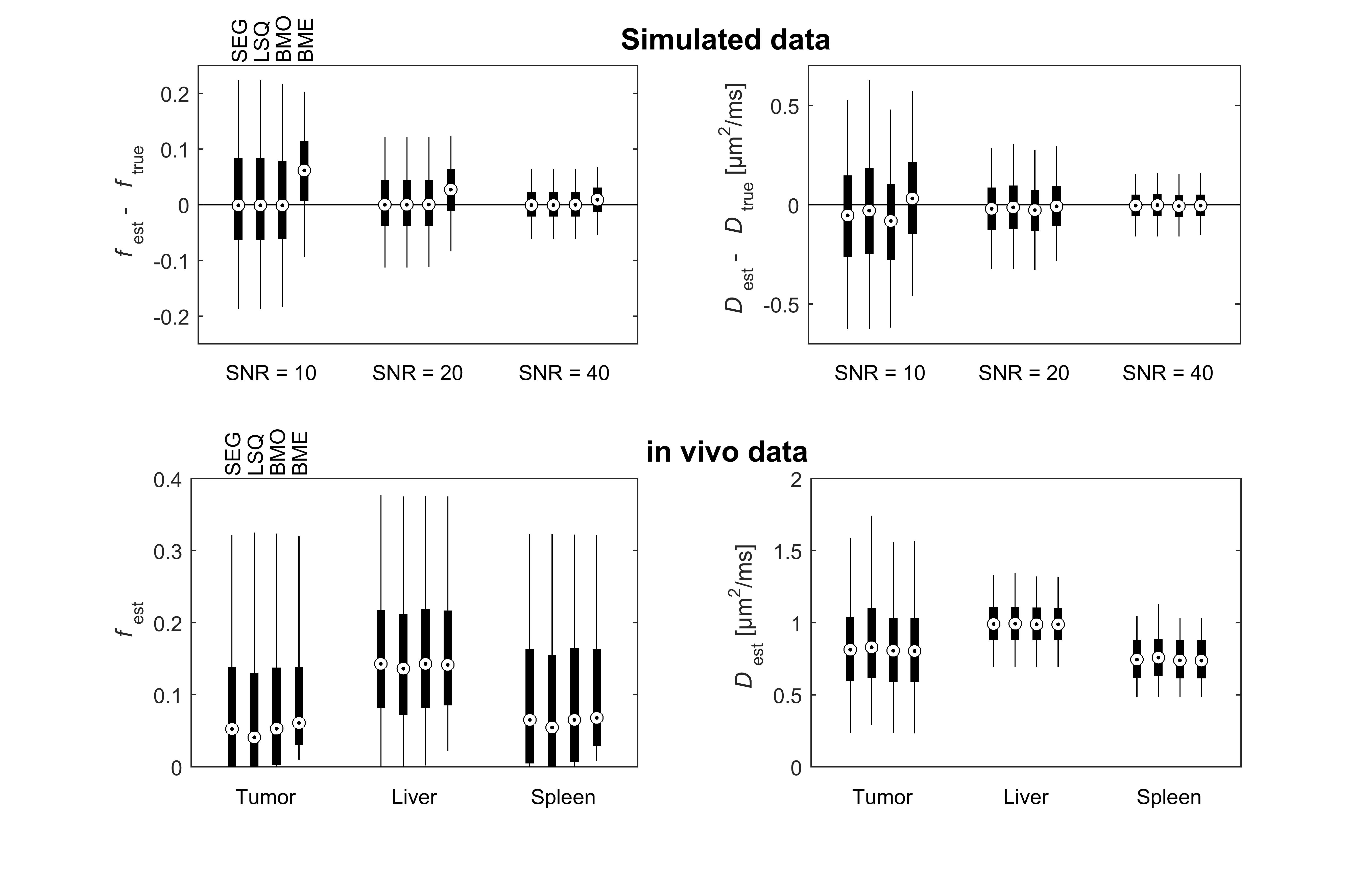
All estimation approaches showed similar performance, with comparable bias and variability, except for the Bayesian posterior mean of f, which had a substantially larger bias (Fig. 1, upper row). The bias of f was only seen if the simulated values of f were small (data not shown). Results from in vivo data agreed well with simulations (Fig. 1, lower row). The biased f was seen for tumor and spleen tissue, but not for liver tissue. This may be explained by the higher f in liver, which gives negligible bias.

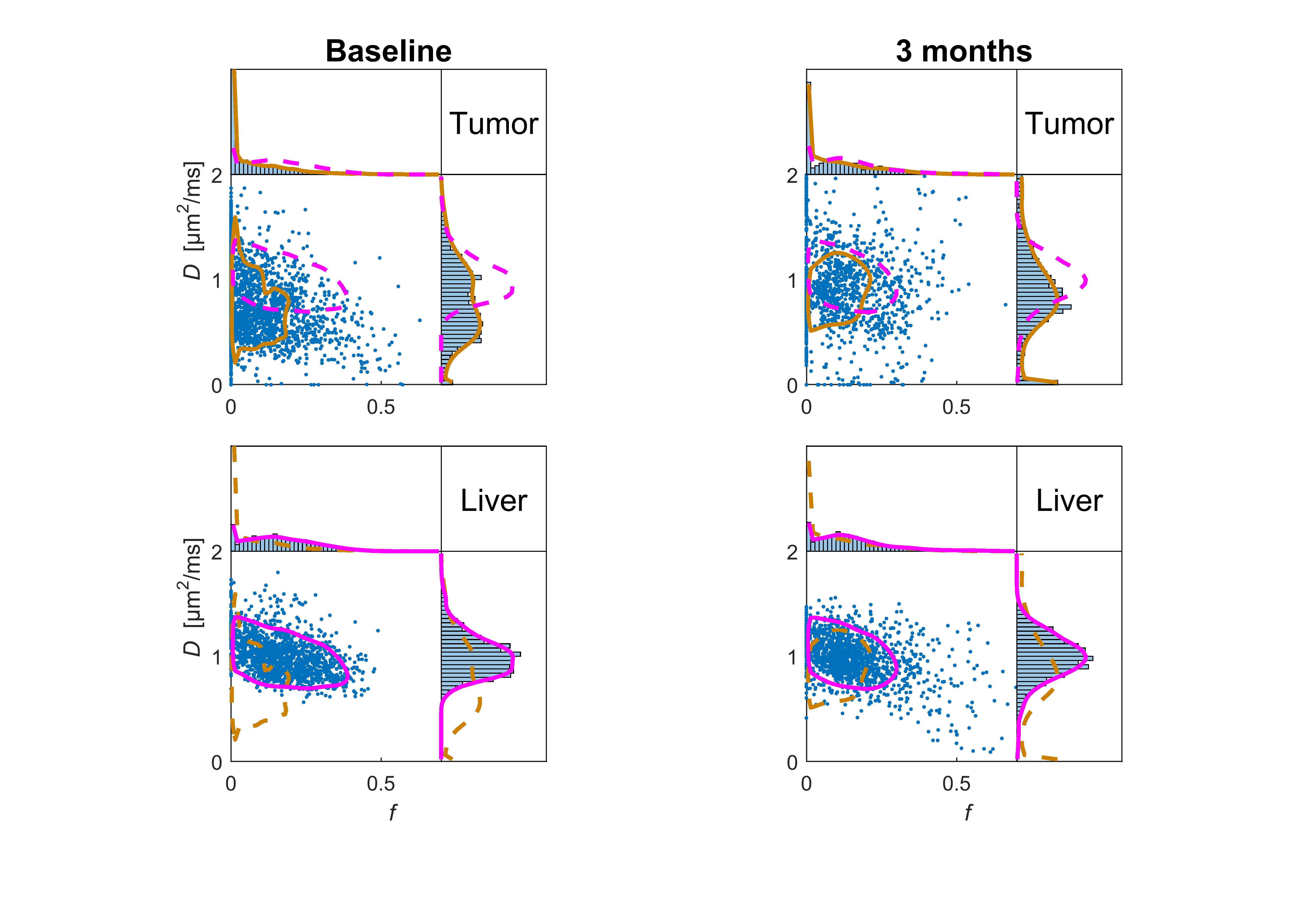
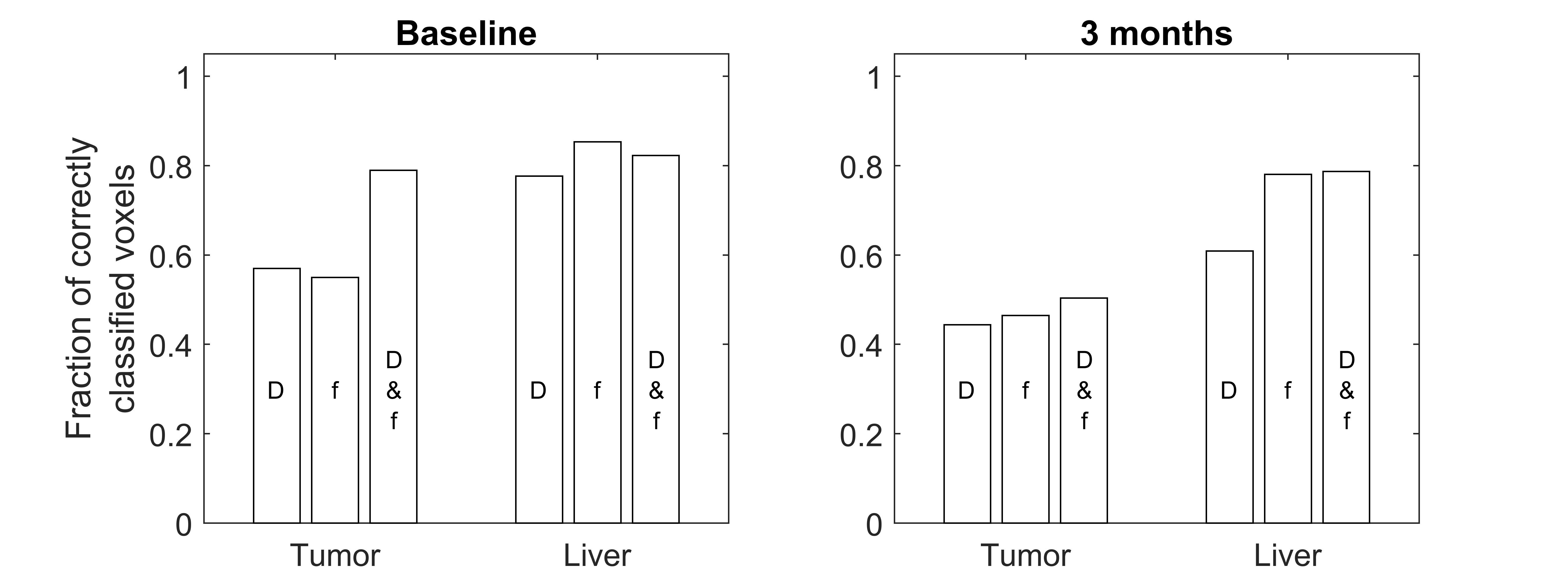
The ability to discriminate between tumor and healthy liver tissue was comparable for all estimation approaches. The distribution of D and f showed a distinct shape for healthy liver tissue whereas the distribution for tumor tissue was more diffuse, especially after treatment (Fig. 2). The ability to differentiate between tumor and healthy liver tissue was enhanced by the combined use of D and f, especially before treatment where it gave specificity and sensitivity of approximately 80% (Fig. 3). The lower classification performance after treatment was likely caused by the mixture of treatments and degree of response.

Conclusions

Acknowledgements

References

1. Le Bihan D, Breton E, Lallemand D, Aubin ML, Vignaud J, Laval-Jeantet M. Separation of diffusion and perfusion in intravoxel incoherent motion MR imaging. Radiology 1988;168:497–505.
2. Padhani AR, Miles KA. Multiparametric Imaging of Tumor Response to Therapy. Radiology 2010;256:348–364.
3. Yuan Q, Costa DN, Sénégas J, Xi Y, Wiethoff AJ, Rofsky NM, Roehrborn C, Lenkinski RE, Pedrosa I. Quantitative Diffusion-Weighted Imaging and Dynamic Contrast-Enhanced Characterization of the Index Lesion With Multiparametric MRI in Prostate Cancer Patients. J Magn Reson Imaging 2016. doi: 10.1002/jmri.25391.
4. Mürtz P, Penner A-H, Pfeiffer A-K, Sprinkart AM, Pieper CC, König R, Block W, Schild HH, Willinek WA, Kukuk GM. Intravoxel incoherent motion model – based analysis of diffusion-weighted magnetic resonance imaging with 3 b -values for response assessment in locoregional therapy of hepatocellular carcinoma. Onco Targets Ther 2016;9:6425–6433.
5. Penner A-H, Sprinkart AM, Kukuk GM, Gütgemann I, Gieseke J, Schild HH, Willinek WA, Mürtz P. Intravoxel incoherent motion model-based liver lesion characterisation from three b-value diffusion-weighted MRI. Eur Radiol 2013;23:2773–2783.
6. Pekar J, Moonen CTW, van Zijl PCM. On the precision of diffusion / perfusion imaging by gradient sensitization. Magn Reson Med 1992;23:122–129.
7. Merisaari H, Movahedi P, Perez IM, et al. Fitting Methods for Intravoxel Incoherent Motion Imaging of Prostate Cancer on Region of Interest Level : Repeatability and Gleason Score Prediction. Magn Reson Med 2016. doi: 10.1002/mrm.26169.
8. Barbieri S, Donati OF, Froehlich JM, Thoeny HC. Impact of the calculation algorithm on biexponential fitting of diffusion-weighted MRI in upper abdominal organs. Magn Reson Med 2016;75:2175–2184.
9. Senegas J, Perkins TG, Keupp J, Stehning C, Herigault G, Smith-Miloff M, Hussain SM. Towards organ-specific b-values for the IVIM-based quantification of ADC: in vivo evaluation in the liver. Proc. Intl. Soc. Mag. Reson. Med. 20 2012. #1891.
10. Yuan Q, Costa DN, Senegas J, Xi Y, Wiethoff AJ, Lenkinski RE, Pedrosa I. A Simplified Intravoxel Incoherent Motion Model for Diffusion Weighted Imaging in Prostate Cancer Evaluation : Comparison with Monoexponential and Biexponential Models.Proc. Intl. Soc. Mag. Reson. Med. 23 2015. #3019.
11. Neil JJ, Bretthorst GL. On the use of Bayesian probability theory for analysis of exponential decay data: an example taken from intravoxel incoherent motion experiments. Magn Reson Med 1993;29:642–647.
12. Gustafsson O, Montelius M, Starck G, Ljungberg M. Impact of prior distributions and central tendency measures on Bayesian intravoxel incoherent motion model fitting. Magn Reson Med 2017. doi: 10.1002/mrm.26783.