Synopsis

The oscillating gradient spin-echo (OGSE) sequence has emerged as a promising diffusion-weighted imaging (DWI) technique for probing in vivo tissue microstructure. However, due to the finite duration of the diffusion gradients, there are some aspects of the signal model that should be considered in more detail. This work re-examines the derivation of the OGSE method to better understand how the properties of the selected MPG are reflected in the signal equation.

Introduction

The oscillating gradient spin-echo (OGSE) sequence has emerged as a promising diffusion-weighted imaging (DWI) technique for probing in vivo tissue microstructure. The theoretical foundations of the technique were first described by Stepisnik [1], but it wasn't until many years later that applications to in vivo brain tissue began [2,3]. Using a notation similar to that in [4], the general signal equation is$$\ln S\left(T\right)=-\frac{1}{2}\int_{-\infty}^{\infty}d\omega\;q\left(\omega\right){\cal D}\left(\omega\right)q\left(-\omega\right)$$where $$$q\left(\omega\right)=\int_0^Tdt\;e^{i\omega T}q\left(t\right)$$$, $$$q\left(t\right)=\gamma\int_0^tdt'\;g\left(t'\right)$$$ and $$$T$$$ is the duration of the motion-probing gradient MPG $$$g\left(t\right)$$$. The dispersive diffusivity $$${\cal D}\left(\omega\right)$$$ is a complex function related to the Fourier transform of the velocity autocorrelation function describing water molecule motion [4]. In the ideal case, the OGSE protocol takes $$$g\left(t\right)=g_0 \cos\omega_n t$$$ (with $$$\omega_n=2\pi n/T$$$) and assumes that the number of oscillations $$$n\gg1$$$. Under these conditions it has been reported that [2-4]$$q\left(\omega\right)=\frac{i\pi\gamma g_0}{\omega_n}\left[\delta\left(\omega-\omega_m\right)-\delta\left(\omega+\omega_m\right)\right],$$ from which it is concluded that the OGSE signal is$$\ln S\left(T\right)\approx-\frac{\gamma^2g_0^2T}{2\omega_n^2}Re{\cal D}\left(\omega_n\right).$$

According to this prescription, the OGSE technique provides a means to directly measure $$${\cal D}\left(\omega\right)$$$ for any medium containing diffusing water molecules. However, we feel that there are some aspects of the derivation that should be considered in more detail. One issue is that the duration of an MPG is limited to around 30-40 ms by the finite transverse relaxation time of brain tissue. As the upper limit on the MPG frequency is around 1 kHz for most current systems, this would mean that the maximum number of oscillations is about 30-40. Unfortunately, this number is limited even further by the fact that the b-value of a cosine MPG is proportional to $$$\left(g_0/\omega_n\right)^2$$$, so that $$$g_0$$$ must be increased to compensate increases in frequency if signal attenuation is to be sufficiently distinguishable from noise. The maximum gradient amplitude available on a standard preclinical system would therefore see the number of oscillations go down to at most 10. For practical application, it is important to clarify whether the limit on the number of oscillations will affect the OGSE signal equation.

A second issue is that, if $$$q\left(\omega\right)$$$ can be written as a sum of two delta functions, from a strict mathematical point-of-view it is not clear how the OGSE signal equation is derived because the square of a delta function is undefined. It seems likely that there is a more subtle relationship between the signal and the spectral properties of the MPG.

Purpose

Results & Discussion

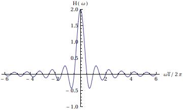
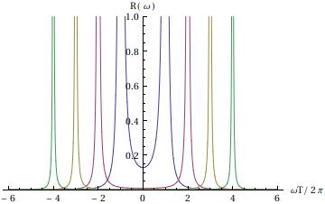
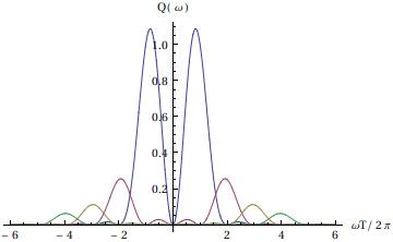
For a cosine MPG, the kernel in the general signal equation is$$Q\left(\omega\right)=q\left(\omega\right)q\left(-\omega\right)=\left(\frac{\gamma g_0}{\omega_n}\right)^2\int_0^Tdt\int_0^Tdt' e^{i\omega\left(t-t'\right)}\sin\omega_n t \sin\omega_n t'.$$ Making the change of variables $$$\tau=t-t', \tau'=t+t'$$$ the kernel becomes$$Q\left(\omega\right)=q\left(\omega\right)q\left(-\omega\right)=\left\{\int_{-T}^0d\tau\int_{-\tau}^{2T+\tau}\!d\tau'+\int_0^Td\tau\int_{\tau}^{2T-\tau}\!d\tau'\right\}e^{i\omega\tau}\sin\frac{\omega_n}{2}\left(\tau+\tau'\right)\sin\frac{\omega_n}{2}\left(\tau-\tau'\right).$$ After some manipulation it can be shown that $$Q\left(\omega\right)=\int_{-T}^Td\tau e^{i\omega\tau}R\left(\tau\right)=\int_{-\infty}^\infty d\tau e^{i\omega\tau}H\left(T-|\tau|\right)R\left(\tau\right)$$ where $$$R\left(\tau\right)=\left(\gamma g_0/\omega_n\right)^2\left[\left(T-|\tau|\right)\cos\omega_n\tau+\omega_n^{-1}\sin\omega_n|\tau|\right]/2$$$ and $$$H\left(t\right)$$$ is the step function. Finally, using the convolution theorem $$Q\left(\omega\right)=\int_{-\infty}^\infty d\omega H\left(\omega-\omega'\right)R\left(\omega\right)$$ with $$$H\left(\omega\right)=2T\mbox{sinc}\omega T$$$ and $$$R\left(\omega\right)=2\left(\gamma g_0\right)^2/\left(\omega^2-\omega_n^2\right)^2$$$. That is, the kernel is the convolution of a sinc function (Fig. 1a) and a function that diverges to $$$+\infty$$$ as $$$\omega\rightarrow\pm\omega_n$$$ (Fig. 1b).

Now, maintaining a finite frequency in the ideal case where the number of oscillations is large (ie $$$n\rightarrow\infty$$$) correspondingly requires that $$$T\rightarrow\infty$$$. In that limit $$$Q\left(\omega\right)=R\left(\omega\right)$$$ so the original equation is $$\ln S\left(T\right)=-\left(\gamma g_0\right)^2\int_{-\infty}^\infty d\omega\frac{{\cal D}\left(\omega\right)}{\left(\omega^2-\omega_n^2\right)^2}.$$ Even though the shape of $$$R\left(\omega\right)$$$ suggests that $$${\cal D}\left(\omega\right)$$$ is only being sampled in a narrow band around $$$\pm\omega_n$$$, more analysis is required to determine the conditions under which the integral is finite. Nevertheless, it is clear that the signal is not simply proportional to $$${\mbox Re}{\cal D}\left(\omega_n\right)$$$.

Acknowledgements

References