1580
q-Space Deep Learning for Alzheimer’s Disease Diagnosis: Global Prediction and Weakly-Supervised Localization1Department of Informatics, Technical University of Munich, Munich, Germany, 2CUBRIC, Cardiff University, Cardiff, United Kingdom, 3Physics Department, Technical University of Munich, Munich, Germany, 4Department of Neurology, University Medical Center Utrecht, Utrecht, Netherlands, 5Image Sciences Institute, University Medical Center Utrecht, Utrecht, Netherlands
Synopsis
Most diffusion MRI approaches rely on comparably long scan time and a suboptimal processing pipeline with handcrafted physical/mathematical representations. They can be outperformed by recent handcrafted-representation-free methods. For instance, q-space deep learning (q-DL) allows unprecedentedly short scan times and optimized voxel-wise tissue characterization. We reformulate q-DL such that it estimates global (i.e. scan-wise rather than voxel-wise) information. We use this formulation to distinguish Alzheimer’s disease (AD) patients from healthy controls based solely on raw q-space data without handcrafted representations such as DTI. Classification quality is very promising. Weakly-supervised localization techniques indicate that the neural network attends to AD-relevant brain areas.
Introduction
Most diffusion MRI approaches rely on relatively long scan time and a suboptimal processing pipeline with handcrafted physical/mathematical representations. They can be outperformed by recent handcrafted-representation-free methods.1,2 For instance, q-space deep learning1 (q-DL) allows unprecedentedly short scan times and optimized voxel-wise tissue characterization.1,2 Here we reformulate q-DL such that it estimates global (i.e. scan-wise rather than voxel-wise) information. We use this formulation of q-DL to distinguish patients with Alzheimer’s disease (AD) from healthy controls based solely on raw q-space data without any handcrafted representations such as diffusion tensor imaging.Methods
Data: The data were as follows:3,4 47 AD patients, 58 healthy controls, one b=0 image (averaged over 3 repetitions), 45 diffusion directions (b=1200s/mm2, single-shot SE-EPI, TR=6638ms, TE=73ms, voxels 1.72mm×1.72mm×2.5mm, matrix 128×128, 48 axial slices), motion/distortion-corrected using ExploreDTI.5 Following deep learning terminology, we refer to each of these 45+1 contrasts (diffusion-weighted images) as “channels”. To study the effect of scan time reduction, separate experiments were performed using sets of 46/30/23/15/7/4 randomly selected channels. For convenient neural network training, so-called feature scaling was performed by dividing each channel by the corresponding channel mean taken over all scans. To prevent overfitting on intensity values, each scan was additionally divided by its mean intensity, and during each training iteration multiplied by a random value between 0.5 and 1.5.
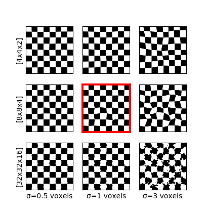
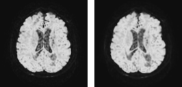
Deformations: For scan-wise AD prediction, we consider each scan a sample (in the machine-learning sense). With a relatively small number of samples (i.e. scans) and large number of features (i.e. voxel values), the neural network would overfit unique but disease-unrelated local image patterns. To circumvent this problem, we generated “additional” images (sized 128×128×48×46) by augmenting the data with random elastic spatial deformations of the original images (sized 128×128×48×46). Thus, the local information varies, while the global context and q-space (important for diagnosis) remain similar. Deformation is done by generating a random coarse 8×8×4 vector grid, upsampling it to 128×128×48 and applying the resulting deformation field to the image. All channels of an image are transformed jointly. Fig. 1 illustrates the influence of the coarse grid parameters. Fig. 2 shows an example on real data.
Network: Five-fold cross-validation was performed: The dataset was split into five equally-sized subsets, and in each fold three of the subsets were used for training, one was used for validation (early stopping) and one for testing (results are reported on the test set of each of the five folds). The neural network architecture was C128-P-C256-P-C512-GP-FC2000-FC1, where Cn is a convolutional layer with n filters sized 3×3×3, P is a 2×2×2 max-pooling layer, GP is a global-pooling layer, and FCn is a fully-connected layer with n units. Hidden-layer nonlinearities: ReLU(z)=max{z,0}, output nonlinearity: sigmoid, trained with binary cross-entropy loss, Adam algorithm,6 learning rate 2·10−5, to distinguish AD patients from healthy controls.
Results
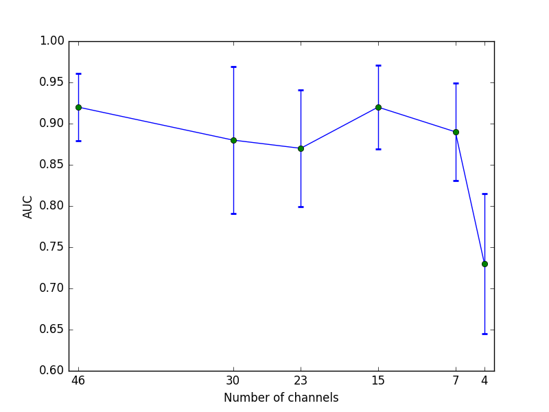
Figure 3 shows the receiver operating characteristic (ROC) for the test sets from the five cross-validation folds. Area under the curve (AUC) in the five cross-validation folds ranges between 0.85 and 0.96. Dependency of AUC on channel number is illustrated in Fig. 4.
Gradient-based class activation mapping7 (Grad-CAM) is a “weakly-supervised localization” technique to visualize on what spatial image area the network bases its decision. Its combination with saliency maps (e.g. guided backpropagation8) that model which inputs strongly influence the prediction, is called Guided Grad-CAM.7 We use these techniques to examine which brain areas drive the network's decision. Visualization of Guided Backpropagation8 and (Guided) Grad-CAM7 for an AD patient that the network correctly classified are shown in Fig. 5.
Discussion
We can thus report that one can train a network directly on q-space data, without any handcrafted representations needed when classifying AD. The network can compensate for missing channels, i.e. providing good predictions for relatively short scan times. AUC drops substantially only when extremely few channels are exposed to the network.
Since the network is able to make good predictions with less channels, it is likely that the essential information is included in few channels. Potentially the network is also able to reconstruct missing information from the exposed subset of channels. Even though the diagnosis was the only output target information available to the network, it seems to focus on brain regions that are prone to AD as can be seen in Fig. 5. This behavior is highly desired since it shows the network’s ability to generalize to unseen data in a meaningful way.
Conclusions
We conclude, (1) that it is possible to directly use raw q-space data as inputs for a convolutional neural network and obtain good classification results when detecting AD, and (2) that the convolutional neural networks seem to learn with weak supervision which areas of the brain are affected by AD.Acknowledgements
This study was partly funded by the European Research Council (ERC Consolidator Grant "3DReloaded"), Deutsche Telekom Foundation, German Research Council (DFG, LA 2804/1-1) and the contribution of Chantal Tax is supported by an FC-EW grant (No. 612.001.104) from the Dutch Scientific Foundation (NWO). The authors would like to thank the members of the Utrecht Vascular Cognitive Impairment Study Group for providing the diffusion MRI data (in alphabetical order by department): University Medical Center Utrecht, the Netherlands, Department of Neurology: E. van den Berg, G.J. Biessels, M. Brundel, W.H. Bouvy, S.M. Heringa, L.J. Kappelle, Y.D. Reijmer; Department of Radiology/Image Sciences Institute: J. de Bresser, H.J.Kuijf, A. Leemans, P.R. Luijten, W.P.Th.M.Mali, M.A. Viergever, K.L. Vincken, J.J.M. Zwanenburg; Department of Geriatrics: H.L. Koek, J.E. de Wit; Hospital Diakonessenhuis Zeist, the Netherlands: M. Hamaker, R. Faaij, M. Pleizier, E. Vriens.References
1. V. Golkov et al. q-Space deep learning: twelve-fold shorter and model-free diffusion MRI scans. IEEE Trans Med Imag. 2016;35(5):1344–1351.
2. V. Golkov et al. Model-free novelty-based diffusion MRI. Proc IEEE Int Symp Biomed Imag (ISBI). 2016:1233–1236.
3. Y.D. Reijmer, A. Leemans, K. Caeyenberghs, et al. Disruption of cerebral networks and cognitive impairment in Alzheimer disease. Neurology 2013;80(15):1370–1377.
4. M. Bach, F.B. Laun, A. Leemans, et al. Methodological considerations on tract-based spatial statistics (TBSS). NeuroImage 2014;100:358–369.
5. A. Leemans, B. Jeurissen, J. Sijbers, D.K. Jones. ExploreDTI: a graphical toolbox for processing, analyzing, and visualizing diffusion MR data. ISMRM 2009:3537.
6. D. Kingma, J. Ba. Adam: a method for stochastic optimization. Proc Int C Learning Representations (ICLR) 2015:arXiv:1412.6980.
7. R.R. Selvaraju et al. Grad-CAM: visual explanations from deep networks via gradient-based localization. Proc Int C Comp Vision (ICCV) 2017:618–626.
8. J.T. Springenberg, A. Dosovitskiy, T. Brox, M. Riedmiller. Striving for simplicity: the all convolutional net. ICLR Workshops 2015.
Figures