1574
Investigating noise distribution changes after motion correction and its effects on subsequent diffusion MRI processingSamuel St-Jean1, Alberto De Luca1, Max A. Viergever1, and Alexander Leemans1
1Image Sciences Institute, Department of Radiology, University Medical Center Utrecht and Utrecht University, Utrecht, Netherlands
Synopsis
The quantification of diffusion MRI assumes the absence of motion and anatomical correspondence between diffusion sensitizing factors. To investigate the impact of processing order between motion correction and two denoising methods, we evaluated DKI and NODDI derived maps. Using repeated scans acquired with and without voluntary motion, three processing orders were compared. Results show that processing order moderately influences NODDI maps. However, two of the three denoising strategies can reduce outliers in mean kurtosis between 28% and 59% when compared to motion correction only.
Introduction
The quantification of diffusion MRI implicitly assumes the absence of motion and anatomical correspondence between diffusion sensitizing factors. To ensure such anatomical correspondence, the diffusion weighted images (DWIs) are corrected for subject motion and eddy current induced distortions1 before further analysis. However, these methods include data interpolation, which changes the underlying statistical profile of the data itself. Various magnitude image reconstruction methods yield different noise distributions2, for which a plethora of specialized estimation methods exist3. Accurate estimation of the noise profile is at the heart of many processing methods, such as denoising4,5, correcting the magnitude signal bias6 or maximum likelihood estimation of biophysical diffusion models7,8, and might influence their outcome. We therefore investigated a) the impact of motion correction on the noise profile and b) if denoising methods or maximum likelihood estimation of diffusion models could benefit from using the original noise profiles.Methods
Two subjects were scanned on a 3T scanner with $$$6\:\text{b}=0\:\text{s/mm}^2$$$ images, $$$8\:\text{b}=500\:\text{s/mm}^2$$$, $$$15\:\text{b}=1000\:\text{s/mm}^2$$$ and $$$32\:\text{b}=2000\:\text{s/mm}^2$$$ for a total of 61 DWIs at $$$\text{TR/TE}=6.5\:\text{s}\:/\:80\:\text{ms}$$$. Three baselines scans and two scans with subject motion (but without signal dropout) were acquired with 2.5 mm isotropic voxel for subject 1 and 2 mm isotropic voxel for subject 2 with an additional $$$\text{b}=0\:\text{s/mm}^2$$$ image and a noise map for each scan (see Figure 1). To assess the impact of motion correction on the noise profile, we tested two publicly available denoising methods, which are MPPCA4 and NLSAM5, using their respective noise estimation procedures and default parameters. Three different cases were investigated: (1) applying motion correction9 before denoising; (2) determining the noise profile, applying motion correction, denoising with the original noise profile and (3) applying motion correction after denoising. For each case, we computed the diffusion kurtosis tensor10 using the REKINDLE algorithm11 as implemented in ExploreDTI12. We then extracted the mean kurtosis (MK) values, which were limited between 0 and 5 to remove physically implausible outliers. We additionally investigated the effect of using either the noise profile as computed before motion correction and after motion correction on a maximum likelihood rician estimator with the NODDI toolbox8. From NODDI, we extracted the intra-cellular volume fraction (ficvf), the orientation dispersion index (odi), the cerebrospinal fluid (CSF) volume fraction (fiso) and the kappa dispersion parameter.Results
Figure 2 shows the empirical noise distribution as measured from the scanner and the histogram of the noise standard deviation from MPPCA and NLSAM. To evaluate the effect of interpolation, each supplementary $$$\text{b}=0\:\text{s/mm}^2$$$ image was registered to the DWIs from the same set. The transformation was applied to the noise map, therefore providing an empirical noise distribution and its modified version due to motion correction. Figure 3 shows the mean kurtosis (MK) maps for one of the scans with both denoising methods and MK maps for the original, motion corrected only datasets for both subjects. For subject 2, applying denoising after motion correction (strategy no. 1) leads to a reduction of 28.23% of outliers for MPPCA and 54.28% for NLSAM when compared to the original, motion corrected only dataset. When applying denoising after motion correction, but using the original noise profile (strategy no. 2), the reduction in outliers increases to 40.31% for MPPCA and 59.09% for NLSAM. Figure 4 shows the relative percentage difference for MK and NODDI maps on all the scans between processing strategies 1, 2 and 3. While denoising and DKI estimation show differences, the maximum likelihood fitting procedure of NODDI seems robust to using either the original noise profile or estimating it after motion correction. Figure 5 shows boxplots of Figure 4 for the MK maps.Discussion & Conclusion
While the empirical noise distribution is undoubtedly modified after registration (see Figure 2), most methods relying on its estimation are also designed to tolerate some misestimation. However, the effects of this misestimation seems to be tied to the signal to noise ratio (SNR) and amount of subject motion present in the data (see Figure 3). For NODDI maps, the largest differences are near CSF, possibly due to partial voluming effect. Regarding denoising, our results suggest that estimating the noise profile on the unprocessed data, then applying motion correction and finally denoising with the original noise profiles can lead to a reduction of 59% in outliers for MK estimates. However, other processing order strategies might improve DKI parameters estimation (see Figure 4). While we only investigated the effects on diffusion MRI, preserving the initial noise distribution for subsequent processing steps could also benefit cardiac MRI or T2w MRI of the abdomen, were involuntary motion is present and motion correction is required.Acknowledgements
Samuel St-Jean is supported by the Fonds de recherche du Québec – Nature et technologies (FRQNT). This research is supported by VIDI Grant 639.072.411 from the Netherlands Organisation for Scientific Research (NWO).References
- Jones, D.K., et al., 2013. White matter integrity, fiber count, and other fallacies: The do’s and don’ts of diffusion MRI. NeuroImage
- Dietrich, O. et al., 2008. Influence of multichannel combination, parallel imaging and other reconstruction techniques on MRI noise characteristics. Magnetic resonance imaging
- Aja-Fernández, S. et al., 2016. Statistical Analysis of Noise in MRI, Cham: Springer International Publishing.
- Veraart, J. et al., 2016. Denoising of diffusion MRI using random matrix theory. NeuroImage
- St-Jean, S. et al., 2016. Non Local Spatial and Angular Matching : Enabling higher spatial resolution diffusion MRI datasets through adaptive denoising. Medical Image Analysis
- Koay, C.G., et al., 2009. A signal transformational framework for breaking the noise floor and its applications in MRI. Journal of magnetic resonance
- Landman, B.et al., 2007. Diffusion tensor estimation by maximizing rician likelihood. Proceedings of the IEEE International Conference on Computer Vision
- Zhang, H. et al., 2012. NODDI: practical in vivo neurite orientation dispersion and density imaging of the human brain. NeuroImage
- Klein, S. et al., 2010. elastix: A Toolbox for Intensity-Based Medical Image Registration. IEEE Transactions on Medical Imaging
- Jensen, J.H. et al., 2010. MRI quantification of non-Gaussian water diffusion by kurtosis analysis. NMR in biomedicine
- Tax, C.M.W., et al., 2015. REKINDLE: Robust extraction of kurtosis INDices with linear estimation. Magn. Reson. Med.
- Leemans A. et al., 2009. ExploreDTI : a graphical toolbox for processing, analyzing, and visualizing diffusion MR data. 17th Annual Meeting of Intl Soc Mag Reson Med
Figures
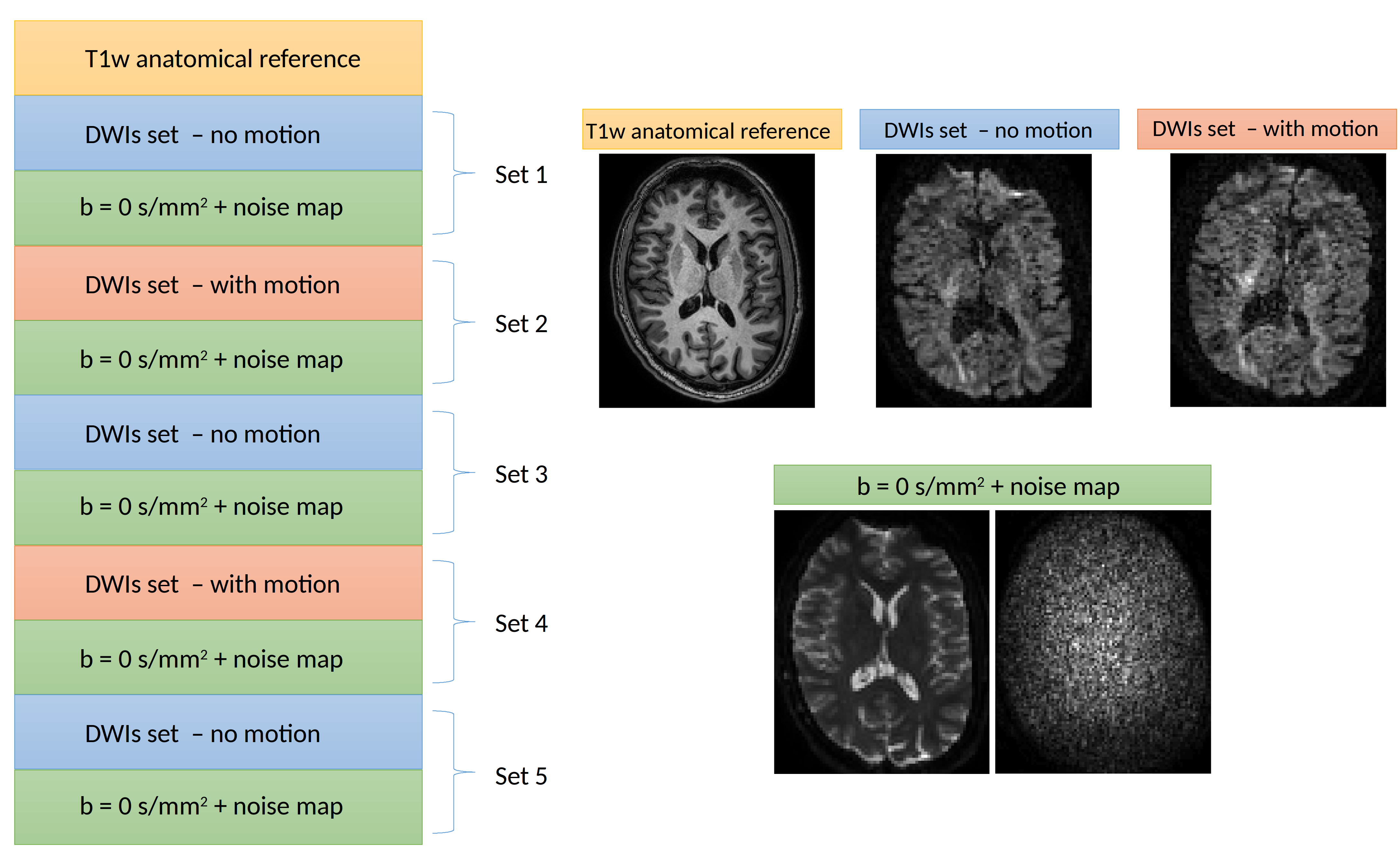
Figure 1 : Schematic of the acquisition protocol. The first scan is established as a baseline without motion, while during the next acquisition block the subjects were allowed to reposition themselves. An additional $$$\text{b}=0\:\text{s/mm}^2$$$ image and a noise map were also acquired after each block. In total, three scans were acquired with subjects laying still and two scans where some movement was present. From the 5 acquisitions of subject 2, we discarded set 2 and set 3 due to acquisition issues.
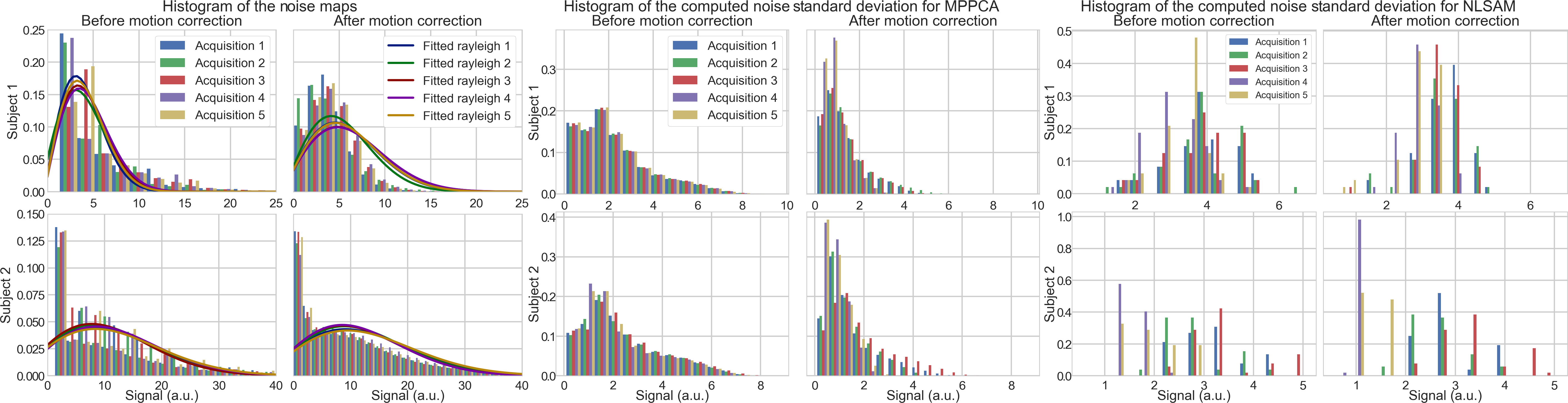
Figure 2 : Normalised histogram before and after motion correction for the raw noise maps with a rayleigh distribution fit (left), noise standard deviation for MPPCA (center) and NLSAM (right). In all cases, the distribution of estimated values is different after applying motion correction. The empirical distribution of the noise maps is altered for both subjects after motion correction. For MPPCA, the estimation is made in 3D local windows and the noise standard deviation is underestimated after applying motion correction. For NLSAM, the slicewise estimation also presents a different profile with most values once again underestimated after motion correction.
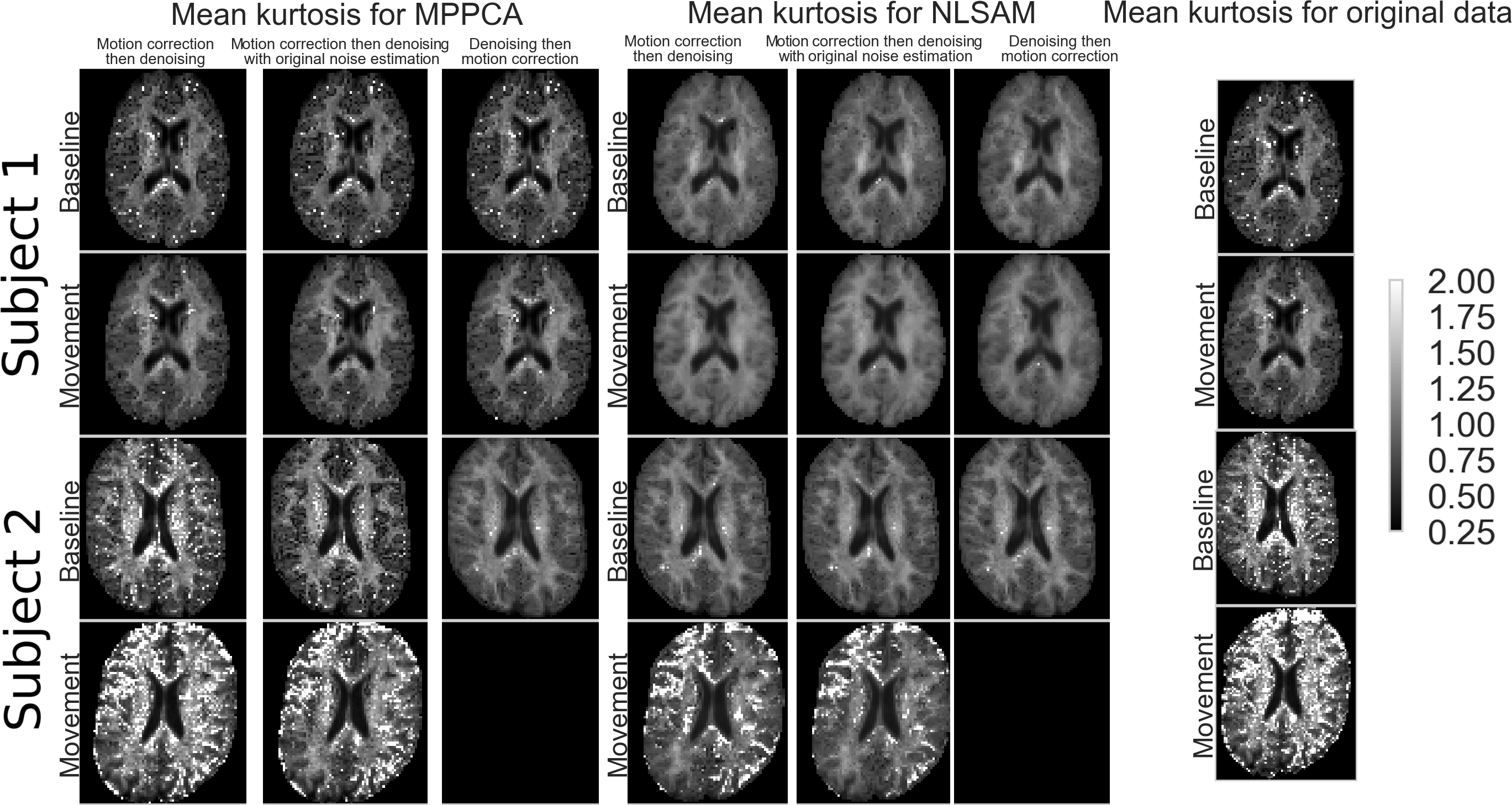
Figure 3 : Mean kurtosis (MK) maps for the three combinations of processing steps for both denoising methods and MK maps of motion corrected data only. A baseline scan (row 1 and 3) and with movement (row 2 and 4) are shown for subject 1 (top) and subject 2 (bottom). Note that less outliers are present in the whole 3D volume when denoising is applied after motion correction, but using the original noise profile (strategy no. 2). This is even more prominent for subject 2, where applying denoising followed by motion correction led to a failure during DKI estimation for the movement dataset.
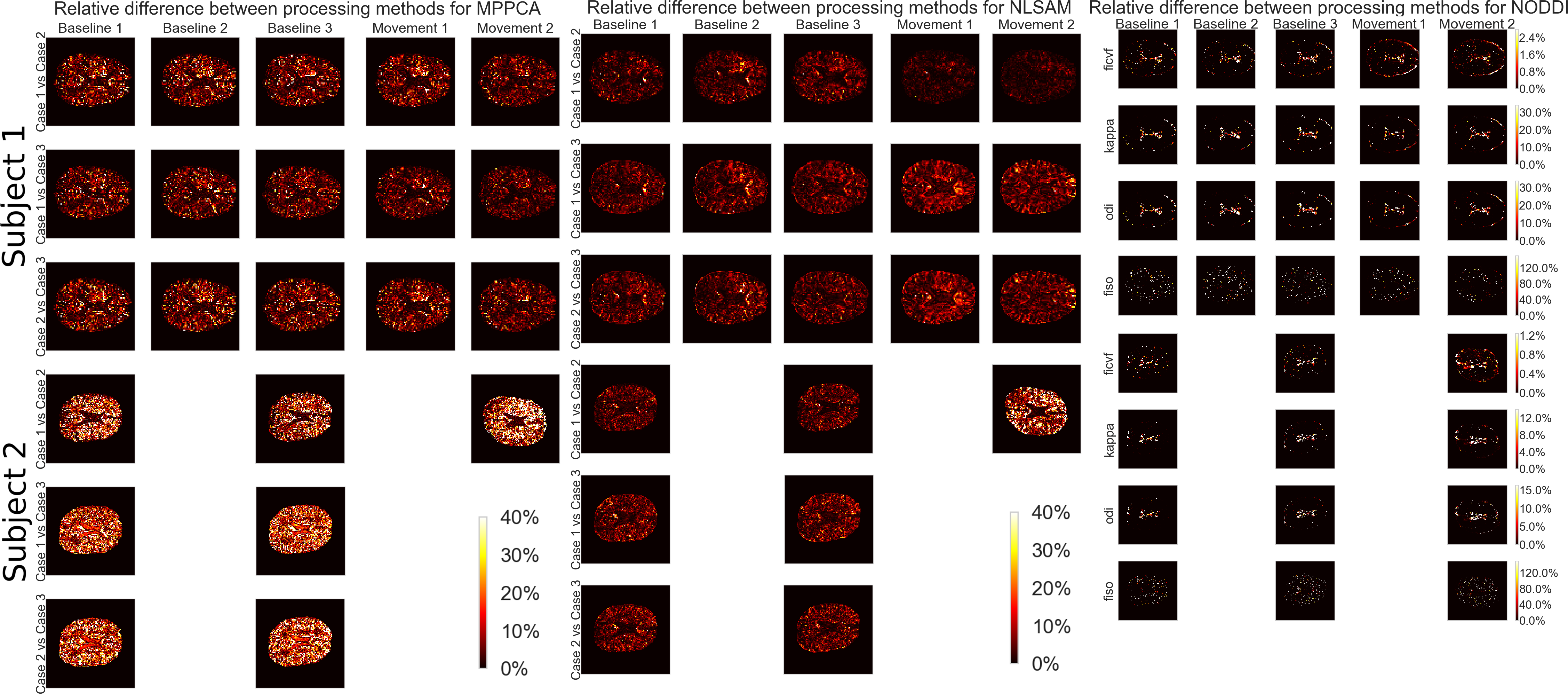
Figure 4 : Relative difference between processing strategies for MPPCA, NLSAM and NODDI. Processing strategies can account for a difference of around 20% for MPPCA and around 10% for NLSAM in the MK estimates. When large subject motion is present (subject 2, movement 2), the difference is almost doubled for both algorithms. In the case of maximum likelihood fitting with NODDI, the results are mostly comparable when using the noise estimates from before or after motion correction, with the largest difference at the outline of the brain or around CSF.
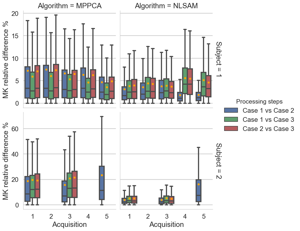
Figure 5 : Boxplot (with the mean as orange dots) of the relative difference MK maps presented at Figure 4 with subject 1 on the top row and subject 2 on the bottom row. For MPPCA, applying denoising before or after motion correction produces less difference in MK values (green boxplots). For NLSAM, using the original noise distribution before or after motion correction (blue boxplots) also yields the smallest difference in MK values. However, while the MK values are different, we do not know yet which strategy yields the smallest error in estimated MK values.