1524
Convolution-Difference Method for Feature Segmentation of Low-Resolution Images1Radiology, University of Miami, Miami, FL, United States
Synopsis
Automated lesion segmentation of clinical imaging studies is of potential value for treatment monitoring and radiation treatment planning. With low spatial resolution imaging systems, such as MR Spectroscopic Imaging, segmentation based on image intensity variations must take into consideration the broad spatial response function. In addition, the relative lesion-to-background intensity variation and the object size must be considered. In this report a new automated image segmentation method is presented that accounts for these factors, which is based on a subtraction of a smoothed version of the MRSI maps from the original data.
INTRODUCTION
Image segmentation based on intensity variations in low spatial resolution imaging modalities, such as MR Spectroscopic Imaging, must consider the spatial response function (SRF) of the imaging system. In addition, the amplitude threshold that provides an accurate volume determination also depends on the relative signal amplitudes in the region to be segmented and the background1,2. In this study, a novel segmentation method is proposed with the aim of addressing these limitations and the performance evaluated using computer simulations and volumetric MRSI data of brain tumors.METHODS
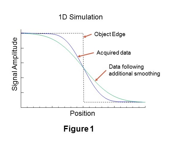
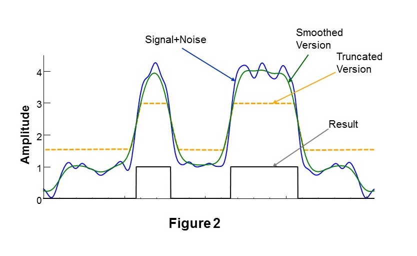
In Figure 1 is shown a simulated one-dimensional cross-sectional profile at the edge of a high signal contrast region (black line). Also shown is the signal, D, that corresponds to the limited k-space sampling of a MRSI dataset with spatial smoothing applied (blue line) and a version of the same signal, D', (green) following additional spatial smoothing. The location of the edge coincides with the position where D=D', and the increased signal region corresponds to where D>D'. This finding must be modified in the presence of noise and Gibbs ringing, as illustrated in Figure 2, which can cause false positives in background regions and false negatives in the high-signal region. It is therefore necessary to modify D' to avoid these ambiguous signal regions, which is done by applying minimum and maximum thresholds, as illustrated by the signal shown in Figure 2 in orange.
The proposed Convolution-Difference segmentation method is therefore as follows:
- Create a smoothed version of the data, D'.
- Find the data value, DC, where D=D'. This is done by taking the derivative of D' and finding the corresponding data value at the location of the maximum of the derivative.
- Truncate D' at a location slightly above DC. A threshold value of DC + 0.25*(D'Max-DC) has been used, where D'Max is the maximum value of D'.
- Based on an initial estimate of the high-signal region, determine the mean, M, and standard deviation, SD, of the background signal. Define a lower intensity threshold as M+4*SD and apply this to D'.
- Apply the logical operation: Result = D GT D'.
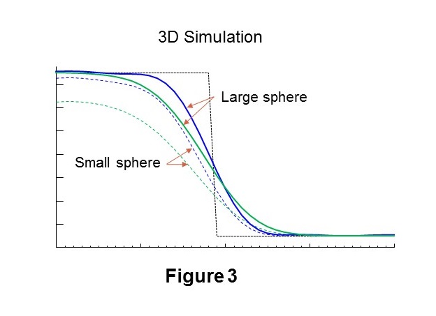
When applied to 3D MRSI the amplitude of D' must be slightly increased to correct for the additive influence of the SRF in multiple dimensions, which is illustrated in Figure 3 using a 3D simulation of two spheres of differing size. In comparison with Figure 1, it can be seen that the location where D=D' no longer corresponds to the edge of the simulated object and that the error is dependent on the object size. The error is also affected by the signal-to-background ratio (SBR). To address this, a scaling factor was determined using a calibration for varying object size and SBR. Since the value of the scaling factor is also dependent on the object size this factor was applied in an iterative manner, using a scaling factor determined from a previous estimate of the object volume and SBR. Typically three iterations were required.
Performance of the proposed segmentation method was evaluated using computer simulation and volumetric MRSI data of brain tumors obtained at TE=70ms.3
RESULTS
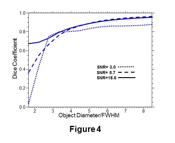
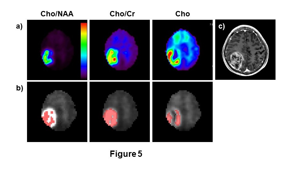
In Figure 4 are shown plots of the Dice coefficient for segmentation of a 3D simulation object defined as a sphere with an intensity gradient, running from 0.5 to 1.0, in one spatial dimension, for three SNR values. Data was simulated for non-isotropic spatial resolution, with 50x50x18 k-space points and nominal voxel size of 5.6x5.6x10 mm3, as is used for a volumetric echo-planar SI acquisition4. In Figure 5 are shown results for a brain tumor segmentation based on the a) Cho/NAA, b) Cho/Cr, and c) Cho signals. Differences in segmentation that reflect different image contrast and heterogeneity in these metabolite maps are apparent.DISCUSSION
The proposed segmentation method represents a novel approach to image segmentation for imaging modalities that have relatively poor spatial resolution. Simulation studies indicate good performance, although degrading for small objects where the object diameter is on the order of the width of the SRF. Preliminary evaluations for volumetric MRSI indicate differing results for segmentation of brain tumors based on maps of Cho/NAA, Cho/Cr, and Cho and further studies are required to determine which if these is the most robust as well as to optimize performance and determine the most suitable MRSI parameters for lesion segmentation.Acknowledgements
This work was supported by NIH grants R01EB016064 and R01CA172210. We thank Dr. R.K. Gupta for acquisition of the data shown in Figure 5.
References
1. Jentzen, W., Freudenberg, L., Eising, E.G. et al. Segmentation of PET volumes by iterative image thresholding. J Nucl Med 2007;48(1):108-114.
2. Zaidi, H., and El Naqa, I. PET-guided delineation of radiation therapy treatment volumes: a survey of image segmentation techniques. Eur J Nucl Med Mol Imaging 2010;37(11):2165-2187.
3. Roy, B., Gupta, R.K., Maudsley, A.A. et al. Utility of multiparametric 3T MRI for glioma characterization. Neuroradiology 2013;55(5):603-613.
4. Maudsley, A.A., Domenig, C., Govind, V. et al. Mapping of brain metabolite distributions by volumetric proton MR spectroscopic imaging (MRSI). Magn Reson Med 2009;61(3):548-559.
Figures