1511
Magnetic resonance fingerprinting on a 1.5T MRI-Linac for tumor response monitoring1Radiotherapy, University Medical Center Utrecht, Utrecht, Netherlands
Synopsis
Magnetic resonance fingerprinting (MRF) is the ideal tool for rapid daily tumor response monitoring on a MRI-Linac (MRL). The 1.5T MRL used in our institution has a modified gradient coil and magnet coil design that potentially complicates the parameter quantification in MRF. In this work we are the first to demonstrate the feasibility of 2D MRF in phantoms and in-vivo on a 1.5T MRL. Moreover, we investigate the accuracy and precision of the parametric maps.
Purpose:
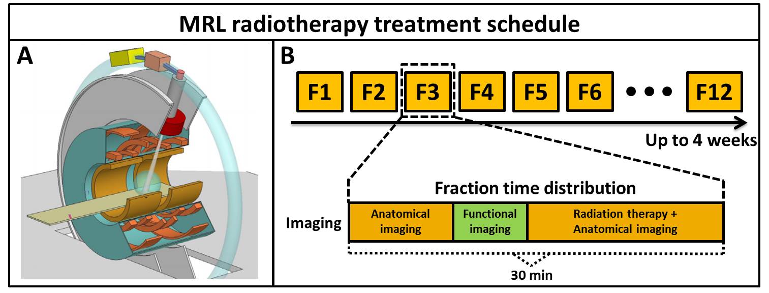
The MRI-Linac (MRL) system will enable (online) daily quantitative tumor response monitoring over the course of the radiotherapy treatment that can be used to adapt the therapy. However, functional imaging time is limited in typical treatment fractions (Fig.1-B) and precise and accurate measurements are essential to steer the therapy based on small changes in quantitative parameter values. Conventional quantitative imaging requires prohibitively long acquisition times for the online setting while simultaneously being sensitive to motion artefacts in the parameter quantification. Magnetic resonance fingerprinting (MRF) enables rapid multiparametric imaging and is therefore the ideal tool for therapy monitoring on the MRL. The 1.5T MRL used in our institution (Unity, Elekta, Crawley, UK) primarily differs from the diagnostic system in the split gradient and split magnet coil design (Fig.1-A). These modifications are expected to affect eddy current behavior and therefore potentially complicate parameter quantification in MRF in terms of accuracy and precision. In this work we are the first to demonstrate the feasibility of 2D MRF in phantoms and in-vivo on a 1.5T MRL and we investigate the accuracy and precision of the parametric maps.Mehods:
Data were acquired using a 2D gradient spoiled MRF sequence with an adiabatic inversion pulse followed by the sinusoidal flip angle train as described previously[2]. One radial line was acquired for every time-point and subsequent readouts were azimuthally incremented using the tiny golden angle to minimize eddy current effects[3]. K-space data and k-space trajectory were corrected using gradient impulse response functions[4]. Tissue fingerprints were simulated with extended phase graphs[5], which included slice profile and B1+. All data were used to estimate the coil sensitivities using ESPIRiT[6] and multi-channel data were combined by multiplication with the complex conjugate of the coil sensitivities[7]. The fully sampled k-space data were reconstructed using the original MRF reconstruction with the maximum correlation method[1], while the retrospectively undersampled k-space data were reconstructed using low rank back-projection[5]. The low rank back projections were subsequently matched with the dictionary to reconstruct the parametric maps.Acquisitions:
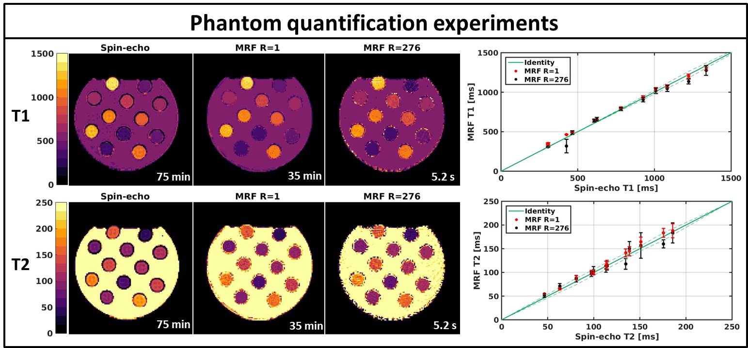
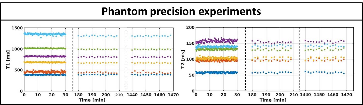
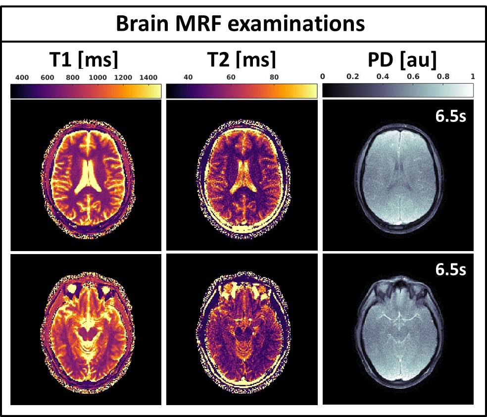
MRF data were acquired on a 1.5T MRL with a 2x4 channel radiation translucent receive array in a phantom and on a healthy volunteer. Reference phantom data were acquired using two separate (inversion recovery and multi echo) spin-echo measurements. Fully sampled MRF phantom data were acquired and were retrospectively undersampled. Phantom experiments were repeated on multiple time-points to quantify the precision of the MRF implementation. Brain and abdominal scans were acquired in a volunteer where the abdominal acquisitions were in breathhold. Acquisition times for a single 2D slice ranged between 5.2s and 6.2s depending on the spatial resolution.Results and Discussion
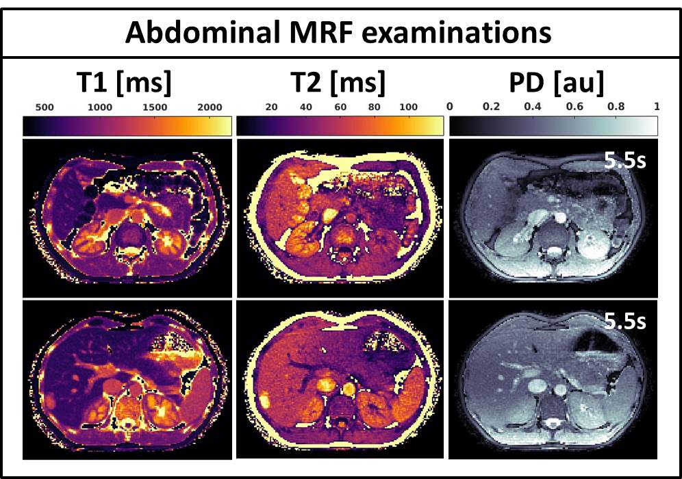
Fig.2 shows the validation of the phantom MRF parameter quantification. The fully sampled (R=1) MRF reconstructions are in good agreement with the gold standard spin-echo quantifications and show high quality parametric maps. The undersampled single spoke (R=276) MRF reconstructions are of similar quality, but slightly underestimate higher T1/T2 values and have higher local standard deviations. Fig.3 shows the mean phantom parameter quantifications for the single spoke MRF reconstructions acquired at multiple time-points. The mean values remain stable over time and have standard deviations of 12ms and 3ms for T1 and T2, respectively. Fig.4 shows the parametric maps of two axial brain images that have good image quality and clear white/gray matter contrast. Fig.5 shows two axial abdominal slices with high quality parametric maps. Note the clear contrast between the renal cortex and the medulla in the T1-map. Validation of the parametric values of the in vivo acquisitions remains future work, but we believe that the results provide strong evidence that 2D MRF is feasible on a 1.5T MRL and has sufficient accuracy and precision to use in a clinical study.Conclusions:
In this work we have shown that 2D gradient spoiled MRF is feasible on a 1.5T MRI-Linac in a phantom and at multiple anatomical locations with good accuracy and precision. The rapid acquisition scheme facilitates an integration into the clinical MRI-guided radiotherapy workflow without significant lengthening of the treatment. These type of acquisitions unquestionably pave the way for multi-parametric quantitative tumor response monitoring and therefore facilitate personalized treatment strategies.Acknowledgements
This work is part of the research programme HTSM with project number 15354, which is (partly) financed by the Netherlands Organisation for Scientific Research (NWO). The authors would like to thank Jakob Asslaender for making the code for the low rank non-uniform FFT operator available online.References
[1] Ma D, Gulani V, Seiberlich N, et al. Magnetic resonance fingerprinting. Nature. 2013;495:187–192.
[2] Jiang Y, Ma D, Seiberlich N, et al. MR fingerprinting using fast imaging with steady state precession (FISP) with spiral readout. Magn. Reson. Med. 2015;74:1621–1631.
[3] Wundrak S, Paul J, Ulrici J, et al. A small surrogate for the golden angle in time-resolved radial MRI based on generalized fibonacci sequences. IEEE Trans. Med. Imaging. 2015;34:1262–1269.
[4] Bruijnen T, Stemkens B, Lagendijk J, et al. Gradient system characterization of a 1.5T MRI-Linac with application to UTE imaging. Proc ISMRM (2018).
[5] Weigel M. Extended phase graphs: Dephasing, RF pulses, and echoes - Pure and simple. J. Magn. Reson. Imaging. 2015;41:266–295.
[6] Uecker M, Lai P, Murphy MJ, et al. ESPIRiT - An eigenvalue approach to autocalibrating parallel MRI: Where SENSE meets GRAPPA. Magn. Reson. Med. 2014;71:990–1001.
[7] Asslaender J, Cloos MA, Knoll F, et al. Low rank alternating direction method of multipliers reconstruction for MR fingerprinting. Magn. Reson. Med. 2017;0:1–14.
[8] McGivney D, Pierre E, Ma D et al. SVD Compression for Magnetic Resonance Fingerprinting in the Time Domain. IEEE Trans. Med. Imaging 2014;62:1–13. doi: 10.1109/TMI.2014.2337321.
Figures